physics613

In this paper, I assume the reader has previously read my other papers on tensors, Lagrangians, and the Standard Model. In this paper, I discuss grand unified theories, supersymmetry, and string theory. I briefly mentioned each of these at the end of my paper on the Standard Model, so I assume the reader has some vague notion of what they are. The Standard Model is a remarkably successful theory. So far, all experimental data is consistent with the Standard Model. However, no one thinks it’s the final theory of nature, since there is so much about it that is unexplained. There are many parameters that have to be added by hand. Why are there three families or generations? Why is charge quantized? The most obvious extension of the Standard Model is grand unification, also called grand unified theory or GUT. This is an attempt to continue the success of the ideas and methods of the Standard Model itself. In the Standard Model, the electroweak theory undergoes spontaneous symmetry breaking, and becomes the electromagnetic and weak force. It’s easy to imagine that some similar method of symmetry breaking of a larger group could give rise to the electroweak and strong gauge groups. Whereas in the Standard Model, the electroweak group SU(2) x U(1) and the QCD group SU(3) are just linked together to form SU(3) x SU(2) x U(1), in grand unified theories, they are all embedded in a larger group, say SU(5). Then quarks and leptons would be placed in the same multiplet, and could be transformed into each other, so baryon number and lepton number are no longer conserved. The idea is to find some way of putting all the various of particles of the Standard Model into a set of multiplets, and write down a Lagrangian that is invariant under the operation of some group G, where G → SU(3) x SU(2) x U(1).

In 1974, Howard Georgi and Sheldon Glashow proposed the SU(5) model, which is the simplest possible grand unified theory. Let’s first address the question, why is SU(5) the simplest group? There are infinitely many Lie groups that could be chosen. There is SU(n), SO(n), Sp(2n), and the exceptional groups which are G₂, F₄, E₆, E₇, and E₈. The order of a group is the number of generators. The rank of a group is the number of generators that can be diagonalized simultaneously. The Standard Model is rank 4, so the group it is embedded in has to be at least rank 4. Also, we want simple groups, meaning groups that aren’t products of other groups. That gives five possibilities, which are SU(5), SO(8), SO(9), Sp(8), and F₄. Now, remember that the Standard Model is parity violating. The left-handed fermions are assigned to doublets, and the right-handed fermions are assigned to singlets. The operation of charge conjugation, which changes the helicity, involves complex conjugation. Real numbers are the same as their complex conjugates, a + 0i = a – 0i, so the group must accommodate complex representations. With this additional requirement, SU(5) is the only group that meets the requirements. The unitary gauge group SU(5) does admit the Standard Model gauge group as the maximal subgroup, and is an ideal candidate for unification. It is the smallest group large enough to contain the Standard Model gauge group. Later, I explain Dynkin diagrams, but suffice it to say here that if you take the diagram for SU(5), and erase the right-most dot, you get the diagram for the Standard Model.

The SU(5) group has 5² – 1 = 24 gauge bosons. Twelve are the familiar gauge bosons of the Standard Model, which are the photon, W⁺, W^–, Z⁰, and the eight gluons. The other twelve gauge bosons change quarks to leptons, and vice versa. The X particles have a charge of -4/3, and the Y particles have a charge of -1/3. Each comes in three colors, red, blue, green, so that’s six. Plus, you have their antiparticles, so that’s twelve. The particles from one family are contained in a mixture of a 5D vector and a 5 x 5 matrix.

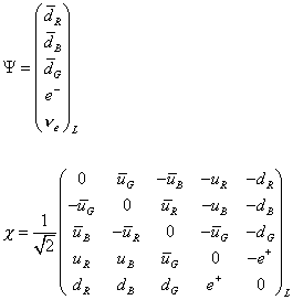
Notice that the above 5 x 5 matrix is an antisymmetric tensor. For a general SU(n) grand unification, in order to ensure the vector nature of the color gauge interactions, to have only three colors, and three anticolors, the simplest choice is to assign fermions only to antisymmetric representations. The irreducible representations will be

[psi]_{i, j, k…}(i, j, k, …) = 1, 2, …n

for SU(n), antisymmetric on exchange of indices. The dimensionality of an mth rank antisymmetric tensor under SU(n) is

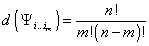
d([psi]_i…im) = n!/m!(n – m)!

This has nothing to do with the dimensionality of spacetime which we’re still assuming is normal 4-D spacetime. You want to have anomaly-free combinations. The anomalies A_m,n associated with an antisymmetric tensor under SU(n) is

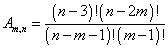
A_m,n = (n – 3)! (n – 2m)/(n – m -1)! (m – 1)!

The formula for the beta function of SU(n) with fermions in [n, m] is

[beta][n, m] = -[(11/3)n – (1/3)[summation][doublet of n-2 m-1] C_m](g³/16[pi]²) + O(g⁵)

The 5D vector I gave earlier is the 5-dimensional representation, and the 5 x 5 matrix is the 10-dimensional representation. If you take both representations as left-handed, as above, so they have the same handedness, the representations are called [5 bar] + 10

meaning the particles in the 5-dimensional left-handed representation are the antiparticles of those in the 5-dimensional right-handed representation. The 5 + 10 representation is

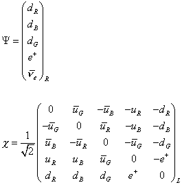
Some people list the colors as 1, 2, 3 instead of R, B, G, or convey antiparticles with a superscript c, meaning charge conjugation, instead of a bar.

You can also have a 24-dimensional representation. A Higgs scalar in the 24-dimensional representation can be used to break SU(5) down to the Standard Model. The 24-dimensional representation is also the adjoint of SU(5) which contains the gauge bosons of the unified group. The theory is specified by writing down the terms of the Lagrangian that couple these fields. The Yukawa coupling can be written down for the fermions in the [5 bar] and 5-dimensional scalar.

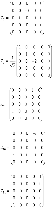
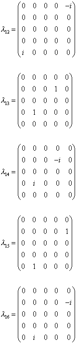
Remember that SU(n) has n² – 1 generators. SU(2) has 2² -1 = 3 generators which are the Pauli spin matrices. SU(3) has 3² -1 = 8 generators which are the Gell-Mann lambda matrices. SU(5) has 5² – 1 = 24 generators. The gauge bosons are added to cancel out the effects of the generators when making the Lagrangian locally invariant. Below are the generators for SU(5). The first eight are just the Gell-Mann matrices in the upper left-hand corner with the rest zero. Matrices 21 – 23 are just the Pauli spin matrices in the lower right with the rest zero. This is similar to the fact that the first three Gell-Mann matrices are just the Pauli spin matrices in the upper left-hand corner with the rest zero. You can guess that the gauge bosons created by the generators that contain the Gell-Mann matrices or Pauli spin matrices are the familiar gauge bosons from the Standard Model.

This gives the following form of the gauge boson matrix. Therefore, the gluons, which are the result of the Gell-Mann matrices, are the 3 x 3 subgroup in the upper left. The photon, W⁺, W^–, and Z⁰, which are the result of the Pauli spin matrices, are in the 2 x 2 subgroup in the lower right.

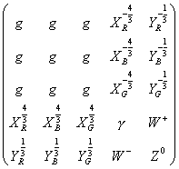
I could have included subscripts for the gluons specifying the color, which are the eight colors I listed in my paper on the Standard Model.

The fact that Standard Model fermions of different charges are accommodated into irreducible representations of SU(5) implies there is a basis for relating the charges of those fermions in the same multiplet. For instance, when we consider the electroweak doublet and the down type antiquark that lie in the same [5 bar], it implies that the action of the same diagonal hypercharge generator produces eigenvalues of their respective hypercharges. This in turn implies that charge is now quantized. Furthermore, we have the result that the normalization of the hypercharge generator is now related to the normalization of the diagonal generators of SU(2) and SU(3).

If you look at the particles in the 5-dimensional representation, their charges add up to zero. This is because, if you notice, the generators of SU(5) are all traceless, meaning of the sum of their diagonals are all zero.

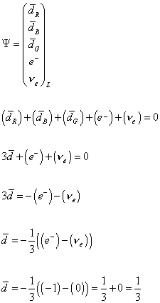
Therefore, the fact that the down quark has exactly 1/3 the charge of an electron, and the fact that hydrogen is electrically neutral, is related to the number of colors of the quarks.

In the Standard Model, you have the Gell-Mann-Nishima relation.

Q = I₃ + Y/2

In SU(5), if we consider the SU(3) subgroup to lie in the upper left 3 x 3 subgroup, and the SU(2) to lie in the lower right 2 x 2 subgroup, then

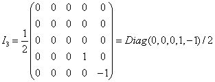
I₃ = Diag (0, 0, 0, 1, -1)/2

and the hypercharge is proportional to

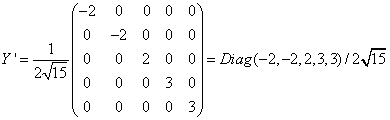
Y’ = Diag (-2, -2, 2, 3, 3)/2[square root of 15]

Therefore, in order to have the correct charge assignments in [5 bar], the 5-dimensional representation, the Gell-Mann-Nishima equation is modified to

Q = I₃ + [square root of 5/3]Y’

Another benefit of SU(5) grand unification is that it accurately predicts the Weinberg angle, θ_w, which is a measure of the ratio of the couplings g₁ and g₂. First, you calculate sin² θ_w at the GUT scale where the symmetry holds, and then you use that to determine what it would be at our energy scale.

Write down the electric charge in terms of the SU(5) generators.

Q = I₃ + cI₁

where I₃ is the SU(2) generator, and I₁ is the U(1) generator. c is a constant. For the SU(5) generators, the covariant derivative is

[partial derivative]^u – ig₅ I_a V_a^u = [partial]^u – ig₅(I₃W₃^u + I₁B^u + …)

where V_a ^u are the SU(5) gauge bosons. There is only coupling constant g₅ for all interactions.

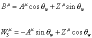
B^u = A^u cos [theta]_w + Z^u sin [theta]_w

W₃^u = -A^u sin [theta]_w + Z^u cos [theta]_w

Therefore you have

-g₅I₃ sin [theta]_w + g₅ sin [theta]_w (I_w – cot [theta]_w I₁) = eQ

Therefore

e = g₅ sin [theta]_w

c = – cot [theta]_w

Now, you have to calculate c from the properties of SU(5). If you take any two generators I_a and I_b, and take the trace of the product, the answer is zero unless a = b. Using Tr I₃ I₁ = 0

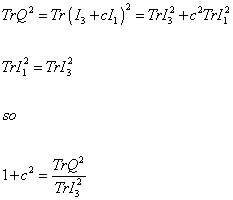
Tr Q² = Tr (I₃ + cI₁)² = Tr I₃² + c² Tr I₁²

Tr I₁² = Tr I₃²

so

1 + c² = (Tr Q²)/(Tr I₃²)

Using the 5-dimensional representation

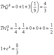
Tr Q² = 0 + 1 + 3(1/9) = 4/3

Tr I₃² = ¼ + ¼ + 0 + 0 + 0 = ½

1 + c² = 8/3

Therefore

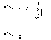
sin² [theta]_w = 1/(1 + c²) = 1/(8/3) = 3/8

However, this is the value predicted for the energy scale at which the GUT symmetry still holds. We now have to calculate it for our energy scale. From the Standard Model Lagrangian

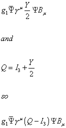
g₁[psi bar] [gamma]^u (Y/2) [psi] B_u

and

Q = I₃ + Y/2

so

g₁[psi bar] [gamma]^u (Q – I₃) [psi] B_u

Also, from the SU(5) Lagrangian

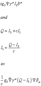
ig₅ [psi] [gamma]^u I₁ B^u

and

Q = I₃ + cI₁

I₁ = (Q – I₃)/c so

(1/c)g₅ [psi bar] [gamma]^u (Q – I₃) [psi] B_u

thus

g₅ = cg₁

[alpha]₅ = c² [alpha]₁

so at the unification scale

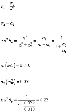
[alpha]₁ = [alpha]₅/c²

[alpha]₂ = [alpha]₅

sin² [theta]_w = g₁²/(g₁² + g₂²) = [alpha] ₁/([alpha]₁ + [alpha]₂) = 1/(1 + ([alpha]₂/[alpha]₁))

[alpha]₁ (m_W²) = 0.010

[alpha]₂ (m_W²) = 0.032

sin² [theta]_w = 1/(1 + (0.032/0.010)) = 0.23

Thus, as you can see, grand unified theory accurately predicts the Weinberg angle, which previously, could only be determined experimentally.

There is indirect evidence for grand unified theory. The coupling constants are not constant but in fact vary with energy. At high energies, which is the same as short distances, they get closer together. The mere fact that they change with energy should not in and of itself suggest that they converge but they do. This suggests that something special does happen when they converge, and we interpret this as the scale at which grand unified theory is broken.

A unification scale M_G ~ 10¹⁶ GeV is suggested by gauge coupling unification, above which physics is described by a grand unified theory based on gauge group G. The arrival at the structure of fundamental interactions from renormalization group flow has a predecessor in the example of asymptotic freedom in deep inelastic scattering experiments, and thus gauge coupling unification is an encouraging sign that grand unified theories are a step in the right direction.

The coupling constants of the Standard Model are logarithmically varying functions of energy described by renormalization group equations of the form

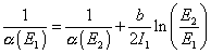
1/([alpha](E₁)) = 1/([alpha](E₂)) + b/(2I₁) ln (E₂/E₁)

where

[alpha] = g²/4[pi]

and the b coefficients are

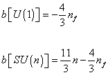
b[U(1)] = -(4/3)n_f

b[SU(n)] = (11/3)n – (4/3)n_f

where n_f is the number of families, which is three in the Standard Model.

If you plot the coupling constants versus energy, you get

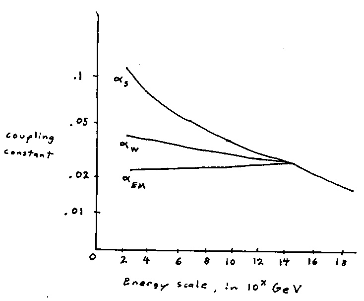
However, despite the fact the coupling constants get closer together, and almost converge, they don’t actually converge. However, if you include supersymmetry, then they do actually converge.

Obviously, the symmetry of SU(5) group is broken at low energies, so we have to figure out how the SU(5) group breaks down to the SU(3) x SU(2) x U(1) group. We do this using the Higgs mechanism, similar to the breaking of electroweak symmetry. We introduce two Higgs multiplets, one belonging to the 24-dimensional representation, called φ, and the other belonging to the 5-dimensional representation, called H. The first stage breaks SU(5) down to the Standard Model, and is given by φ not being zero. The second stage breaks the electroweak, and is given by H not being zero.

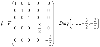
[phi] = V Diag (1, 1, 1, -3/2, -3/2)

The breakdown is along the λ₂₄ direction. This is responsible for the first stage of symmetry breaking. The second stage is given by

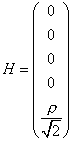
In the presence of both H and φ, the vacuum expectation value of φ changes to

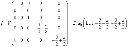
[phi] = V Diag (1, 1, 1, -3/2 – [epsilon]/2, -3/2 + [epsilon]/2)

Therefore, the masses of bosons are

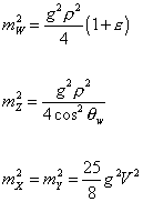
m_W² = (g²p/4)(1 + [epsilon])

m_Z² = g²p/4 cos² [theta]_w

m_X² = m_Y² = (25/8)g²V²

You also have to add several Higgs multiplets to generate the fermion masses. The part of the Lagrangian that involves X and Y is

L_{X, Y} = (ig_X/[square root of 2]) X_u,i ([epsilon]_ijk [u bar]_kL [gamma]_u u_jL + [d bar]_i [gamma]_u e⁺) + (ig_Y/[square root of 2]) Y_{u, i} ([epsilon]_ijk [u bar]_KL [gamma]_L d_hL – [u bar]_iL e⁺_L + [d bar]_iR [gamma]_u [nu bar]_R) + hermitian conjugate

The Hamiltonian obtained for X and Y exchange for the first generation is

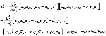
H = (g_X²/2M_X²) [[epsilon]_ijk [u bar]_kL [gamma]_u u_jL + [d bar]_i [gamma]_u e⁺] [[epsilon]_ilm [u bar]_lL [gamma]_u [u bar]_mL + e⁺ [gamma]_ud_I] + (g_Y/2M_Y²) [[epsilon]_ijk [u bar]_kL [gamma]_u d_jL – [u bar]_iL [gamma]_u e⁺_L + [d bar]_iR [gamma]_u [nu bar]_R] x [[epsilon]_ilm [d bar]_lL [gamma]_u [u bar]_mL – e⁺_L [gamma]_u u_iL + [nu bar] [gamma]_u d_IR] + Higgs contributions

Some people call the X and Y bosons leptoquarks, since they mediate reactions that convert leptons to quarks, and vice versa, but I think this is a misleading name, since it implies they are similar to leptons and quarks. X and Y bosons are bosons, and are thus totally different from leptons and quarks, which are fermions.

The exchange of X and Y bosons allows new reactions to take place. These reactions would take place much more rarely than the Standard Model reactions because the X and Y bosons have masses on the order of the GUT scale, and thus would be very short range. It’s rare that two particles would stray close enough to each other to exchange one. However, when they do, a quark can be converted into a lepton, or vice versa. Here are the vertices that can be used to construct Feynman diagrams.

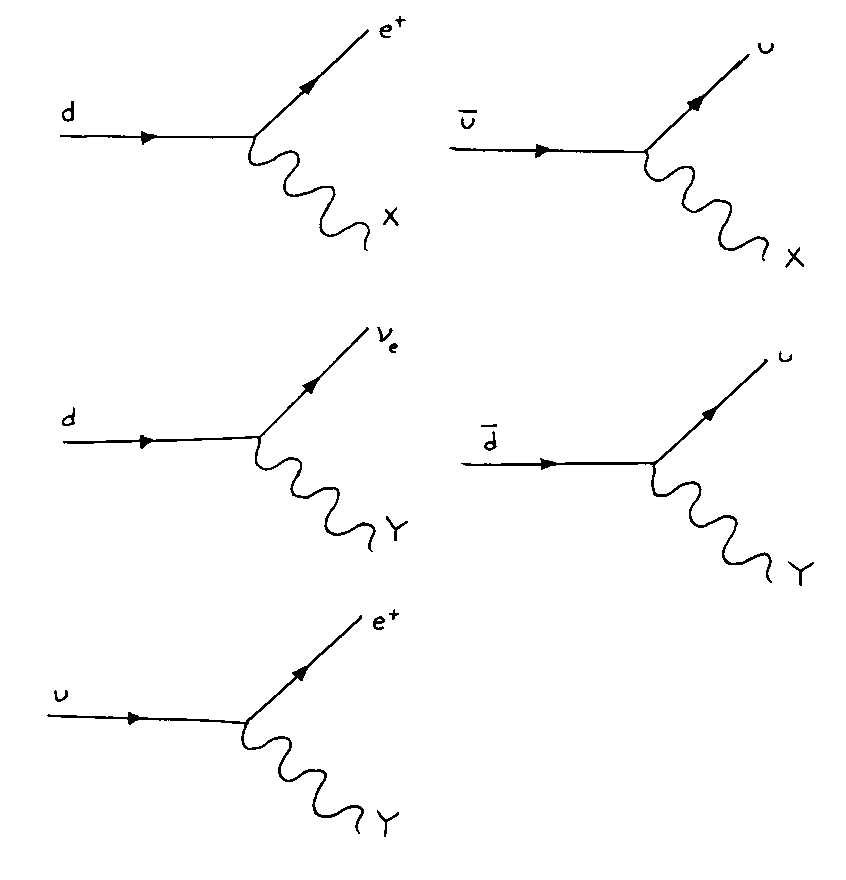
The fact that you can now convert quarks to leptons, and baryon number is no longer conserved, means that the proton is no longer absolutely stable. Here are some possible decay modes for the proton.

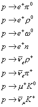
p -> e⁺ [pi]⁰
p -> e⁺ [rho]⁰
p -> e⁺ w⁰
p -> e⁺ n
p -> [nu bar] [rho]⁺
p -> [nu bar] [pi]⁺
p -> [mu]<⁺ K⁰
p -> [nu bar]_[mu] K⁺

The last one involves flavor mixing effects. Similarly, a bound neutron inside a nucleus can now decay, via the following decay modes.

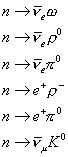
n -> [nu bar] w
n -> [nu bar] [rho]⁰
n -> [nu bar] [pi]⁰
n -> e⁺ [rho]^–
n -> e⁺ [pi]⁰
n -> [nu bar]_[mu] K⁰

The last one involves flavor mixing effects. It should be noted that even though baryon number and lepton number are not conserved, baryon number minus lepton number, B – L, is conserved. The X and Y bosons have a definite B – L of 2/3.

The most common way for a proton to decay is by p → e⁺ π⁰

There are several different diagrams that correspond to this reaction but the most common ways for it to happen is by either of the following two diagrams.

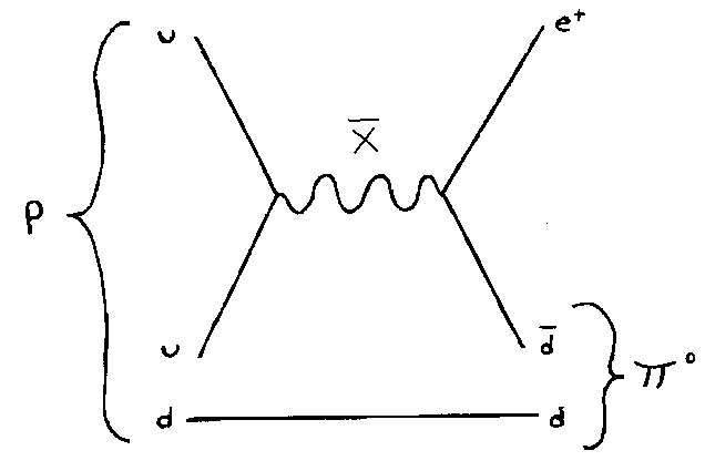
as well as

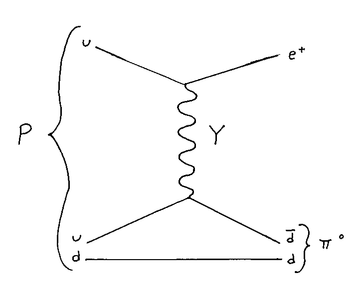
Branching ratios are a measure of what percentage of decays are by a given decay route.

p → e⁺ π⁰ would have a branching ratio of 40% – 60%.

p → e⁺ w would have a branching ratio of 5% – 20%.

p → e⁺ ρ⁰ would have a branching ratio of 1% – 10%.

p → [ν bar]_e π⁰ would have branching ratio of 16% – 24%.

The cross section for p → e⁺ π⁰ is given by

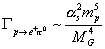
[capital gamma] ~ ([alpha]_s² m_p²)/M_G⁴

The smaller the cross section, the more rare two particles will be that close, and so the lifetime is the inverse of the cross section.

We aren’t that sure of the exact value of the GUT scale, but if you plug in the common range of values, you get 10³⁰ – 10³¹ years.

Since the Universe is only 13.7 billion years old, you might think it would be impossible to detect this. However, by looking at a large number of protons, you could theoretically detect this. One cubic centimeter of water contains 6 x 10²³ nucleons, so a cube 10 meters on a side contains 10³³ nucleons. Therefore, by looking at 10,000 tons of water, you should be able to detect proton decay. The signature of p → e⁺ π⁰ decay is photons since π⁰ → γ γ, and e⁺ gives Cerenkov radiation. The detector must be sensitive to very few photons, and the water must be so pure that a decay anywhere will be visible to the photomultiplier tubes on the walls.

Such proton decay detectors have been looking for proton decay for the past 15 years. During that time, they have been very successful at detecting neutrinos, such as from Supernovae 1987A or from the Sun, establishing the solar neutrino problem, which is strong evidence that neutrinos have mass. However, there has never been a confirmed signal of proton decay. In other words, SU(5) grand unified theory has been ruled out experimentally. Although initially disappointing, this really shouldn’t be all that surprising, since SU(5) is the only the simplest possible extension of the Standard Model. I don’t think anyone seriously thought that SU(5) all by itself was the final theory in physics. Higher gauge groups in grand unified theories, such as SO(10), can predict longer proton lifetimes. Also, if you combine grand unified theories with supersymmetry, it predicts a proton lifetime of 10³³ years which has not been ruled out by experiment. Today, particle physicists always include supersymmetry in their models, and in that case, it would probably be impossible to confirm the prediction of proton decay. Probably the upper limit on what can be detected is 10³² years. Beyond that level, intrinsic backgrounds that look just like the signal are too frequent to allow a signal to be seen. Such backgrounds could arise from say, an upper atmosphere cosmic ray collision that produces pions, which then decay to neutrinos, followed by neutrino interactions that produce the same final signature as a real decay, and can’t be separated by analysis. Since supersymmetric grand unified theories predict a proton lifetime of 10³³ years, that pretty much rules out detecting proton decay as a possible way of confirming the model.

This does lead to a more general criticism of post-Standard Model physics, which is its lack of connection with experiment. From when Han Oersted noticed that an electric current deflects a compass needle in 1819, the first indication of a connection between electricity and magnetism, to the detection of the W⁺, W^–, and Z⁰ bosons with the predicted masses at CERN in 1983, the progress of particle physics has been an enthusiastic rush of both theoretical and experimental advancement, inextricably intertwined, as theoretical predictions were immediately confirmed by experiment, and experimental puzzles were quickly explained by new theories. However, theory and experiment drifted apart after the detection of the W⁺, W^–, and Z⁰. Of course, there have been great experimental successes of particle physics since then, such as the detection of the top quark in 1995, and the tau neutrino in 2000. However, these were still just confirmations of the Standard Model, which modern theoretical particle physics considers as quaint as Newtonian mechanics. Since then, particle physics has moved far beyond the Standard Model, into the realm of grand unification, supersymmetry, and string theory, none of which are directly experimentally testable with current technology. This has led to a totally unfair criticism of particle physics. John Baez, another physics writer on the Internet, wrote about the failure to detect proton decay, “Theoretical physics never really recovered from this crushing blow. In a sense, particle physics gradually retreated from the goal of making testable predictions into a wonderland of pure mathematics, first supersymmetry, then supergravity, then superstrings, even more elegant theories, but never a verified experimental prediction.”

This is a totally unfair criticism. If there was experimental evidence against modern theories, then that would be a criticism of them. However, there is currently no experimental evidence either for or against them, since they discuss phenomena that exist at higher energies than we can currently reach in our particle accelerators. Second of all, there is evidence, maybe not direct experimental evidence, but indirect evidence for them, which is that they successfully explain whatever unexplained aspect of the Standard Model or the Universe that they were invented to explain in the first place. Third of all, John Baez and people like him seem to miss the point of what is the purpose of physics. We’ll never know the real truth about what is the real Universe at the most fundamental level. All theories in physics are invented by people as attempts to possibly explain unexplained aspects of what we observe, or unexplained aspects of previous theories. We’ve never had a theory or view of the Universe that was totally true, and we never will. That’s not the purpose of physics. The purpose of physics is to explain what you observe. If you think up a theory that has some unexplained aspect or parameter, then you have to try to think up something that could possibly explain it, such as how SU(5) was able to explain the quantization of charge, or predicted the Weinberg angle. By that standard, the extensions of the Standard Model, such as grand unification, supersymmetry, or string theory, are as successful as any theory we’ve ever had in physics, and there is not a shred of experimental evidence against them. The only thing the critics could point to is the lack of detection of proton decay, which only ruled out the simple SU(5) model all by itself, which no one seriously thought was the ultimate description of nature anyway. Even if these theories turn out not to be true, so what? They explained what they were intended to explain, and were consistent with all experimental data that existed at the time of their invention, which is the most anyone could ask of any theory. We’ve never had a theory that was actually true, and we never will. For instance, Newtonian mechanics is obviously not true, since it doesn’t take into account relativity or quantum mechanics. Is that a valid criticism of Newton?

Even before SU(5) was ruled out experimentally, people were looking at other grand unified theories. In 1974, Howard Georgi and Sheldon Glashow proposed SU(5). In 1975, Georgi proposed embedding SU(5) in a larger gauge group called SO(10). Actually, the idea of using the SO(10) group actually occurred to him a few hours before he realized that you could contain the Standard Model within the simpler SU(5) group. The SO(10) model was also proposed independently by Fritzsch and Minkowski in 1975. The SU(5) model we’ve been discussing still exists, just embedded within a larger group called SO(10). Therefore, SO(10) contains SU(5), which contains the Standard Model, SU(3) x SU(2) x U(1), which contains QCD, SU(3), and the electroweak, SU(2) x U(1), which contains QED and the weak force. Our theories in particle physics end up being like nestled Russian matryoshka dolls, with each group nestled within a larger one. The main criticism of SU(5) is that it didn’t unify all the fermions of a given generation in a single irreducible representation, together with its dual for antiparticles. SO(10) solves this problem, and contains SU(5) as a subalgebra, with SU(5) x U(1) being the maximal subalgebra. The SU(5) subgroup can be the Georgi-Glashow SU(5) model but it doesn’t have to be. You could use a different SU(5). You could choose a linear combination of one of the diagonal generators of SU(5) and the additional U(1) of the maximal subalgebra as the hypercharge. This is called flipped unification, referring to the flipping of the assignments of certain particles to representations of the SU(5) model. SO(10) is in a class of groups that admit spinor representations of dimension 16. Remember that SU(5) is 15-dimensional, so here there is an additional 16th state, which is identified with the right-handed neutrino. Remember that the Standard Model has only left-handed neutrinos. The 16-dimensional representation is an obvious candidate for Standard Model generation, and in addition, contains a candidate for a right-handed neutrino, which is a SU(5) singlet. Remember that in the Standard Model, the absence of a right-handed neutrino means there is no obvious way to give masses to the neutrinos. In SO(10), the presence of a right-handed neutrino means you can easily give masses to the neutrinos, which is an obvious benefit to the theory.

SO(10) is actually a combination of the two simplest extensions of the Standard Model, one being SU(5), and the other being the left-right symmetric model. This model was invented to explain parity violation, which is one of the unexplained aspects of the Standard Model. Weak interactions are parity violating, but this has to be added to the theory in an ad hoc way. The Standard Model does not address the question of why nature is parity violating. The left-right symmetric model explains this by suggesting that the Standard Model is embedded in a higher gauge group that is parity conserving. Then through symmetry breaking, it reduces to the smaller subgroup which survives to low energies, and is parity violating. The left-right symmetric model is perhaps more accurately described as an extension of electroweak theory. At high energies, the gauge group is SU(2)_L x SU(2)_R x U(1)_{B – L}, and at low energies, it reduces to the SU(2)_L x U(1) group of electroweak theory. The SU(3) group of the strong force is carried along unaffected by this symmetry breaking. One interesting thing is that the U(1) group of the Standard Model is now associated with the B – L quantum number, which is baryon number minus lepton number. This model predicts that at high energies, when the symmetry is unbroken, you should see effects associated with parity conservation, such as the right-handed neutrino, right-handed charged currents, and a second neutral Z⁰ boson. The left-right model allows for a right-handed neutrino, and thus neutrino mass. It makes the weak force more similar to the strong force, so the forces are more consistent, and more unified. It provides a possible interpretation of the U(1) group. It can also provide an alternative explanation for CP-violation, other than the KM-matrix. In the Standard Model, the Gell-Mann-Nishima relation is

Q = I₃ + Y/2

In the left-right symmetric model, this is modified to

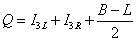
Q = I_3L + I_3R + (B – L)/2

SO(10) is then a combination of the SU(5) model with the left-right symmetric model, having the benefits of each. Unlike SU(5) which is rank 4, SO(10) is rank 5 with the extra diagonal generator of SO(10) being B – L, as in the left-right symmetric model. The advantage of SO(10) over SU(5) as the group for grand unification is one 16-dimensional spinor representation of SO(10) has all the right quantum numbers to accommodate all the fermions, including the right-handed neutrino, of one generation. The gauge interactions of SO(10) conserve parity, thus making parity a continuous symmetry. Aside from providing a reason of why and how parity is violated in the Standard Model, it helps avoid the cosmological domain wall problem. SO(10) is the minimal left-right symmetric grand unified theory that gauges the B – L symmetry, and is the only simple grand unified group that does not need mirror fermions. The model does not have any global symmetries. Here are the different possible dimensional representations of SO(10), and their decomposition to irreducible multiplets. These are called branching ratios.

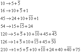
10 -> 5 + [5 bar]
16 -> 10 + [5 bar] + 1
45 -> 24 + 10 + [10 bar] + 1
54 -> 15 + [15 bar] + 24
120 -> 5 + [5 bar] + 10 + [10 bar] + 45 + [45 bar]
126 -> 1 + [5 bar] + 10 + [15 bar] + 45 + [50 bar] 210 -> 1 + 5 + [5 bar] + 10 + [10 bar] + 24 + 40 + [40 bar] + 75

Here are the various ways in which the SO(10) group can break down to the lower subgroups.

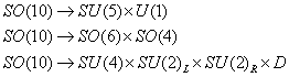
SO(10) -> SU(5) x U(1)

SO(10) -> S0(6) x SO(4)

SO(10) -> SO(4) x SU(2)_L x SU(2)_R x D

where D is the discrete symmetry of charge conjugation.

q_L -> [q bar]_L

The following is one way to define the algebra of SO(10). Let’s say you have a set of operators X_i ( i = 1, 2…n) and their hermitian conjugate X_i^†, satisfying the following anticommutation relation.

{ X_ij, X_j^†} = [delta]_ij

{X_i, X_j} =0

The operators T_jⁱ are defined as

T_jⁱ = X_j^† X_j

satisfy the algebra of the U(n) group

[T_jⁱ, T_l^k] = [delta]_j^k T_lⁱ – [delta]_lⁱ T_j^k

Let’s define the following 2n-operators

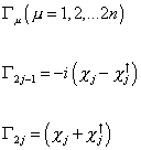
[capital gamma]_u (u = 1, 2…2n)

[capital gamma]_{2j – 1} = -I(X_j – X_j^†)

[capital gamma]_2j = (X_j + X_j^†)

where j = 1, 2,…n

Therefore

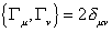
{[capital gamma]_u, [capital gamma]_v} = 2[delta]_uv

Therefore, the Γ_u‘s form a Clifford algebra of rank 2. Also

[capital gamma]_u = [capital gamma]_u^†

Therefore, using the Γ_u‘s, we can construct the generators of the SO(2n) group as follows

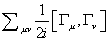
[capital sigma]_uv = (1/2i)[[capital gamma]_u, [capital gamma]_v]

The Σ_uv can be written down in term of X_j and X_j^† as follows.

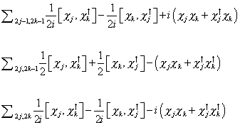
[capital sigma]_{2j – 1, 2k – 1} = (1/2i) [X_j X_k^†] – (1/2i)[X_k, X_j^†] + I(X_jX_k + X_j^†X_k)

[capital sigma]_{2j, 2k – 1} = (1/2) [X_j X_k^†] + (1/2)[X_k, X_j^†] – (X_jX_k + X_j^†X_k^†)

[capital sigma]_{2j, 2k} = (1/2i) [X_j X_k^†] – (1/2i)[X_k, X_j^†] – I(X_jX_k + X_j^†X_k^†)

The spinor representation of SO(2n) is 2ⁿ dimensional. Let’s define a vacuum state |0> that is SU(n) invariant. The 2ⁿ dimensional representation is then given by

X₁^† X₂^† … X_n^† |0>

This representation can be split into the 2^{n – 1} dimensional representation by using a chiral projection operator. To construct this operator, define

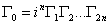
[capital gamma]₀ = iⁿ [capital gamma]₁ [capital gamma]₂… [capital gamma]_2n

Also define the number operator

n_j = X_j^† X_j

Γ₀ can be written as

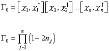
[capital gamma]₀ = [X₁, X₁^†] [X₂. X₂^†] …[X_n, X_n^†]

[capital gamma]₀ = [product of j – 1 to n](1 – 2n_j)

Since the number operator satisfies n_j² = n_j, you have

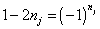
1 – 2n_j = (-1)^n_j

so therefore you have

[capital gamma]₀ = (-1)ⁿ

n = [summation of j] n_j

so then you have

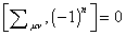
[[capital sigma]_uv, (-1)ⁿ] = 0

so then the chirality projection operator is given by

(1/2)(1 ± [capital gamma]₀)

Each irreducible chiral subspace is therefore characterized by either an odd or even number of X particles.

We are constructing the spinor representation of SO(2n) that includes SU(n). Since we want specifically to write down the representation of SO(10) that includes SU(5), lets say n = 5. Also, let’s define a column vector | Ψ > such that

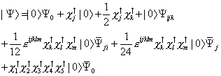
| [psi] > = | 0 > [psi]₀ + X_j^† | 0 > + (1/2) X_j^† X_k^† + | 0 > [psi]_ijk + (1/12) [epsilon]^ijklm X_k^† X_l^† X_m^† | 0 > [psi bar]_ji + (1/24) [epsilon]^jklmn X_k^† X_l^† X_m^† X_n^† | 0 > [psi bar]_j + X₁^† X₂^† X₃^† X₄^† X₅^† | 0 > [psi bar]₀

where [psi bar] is not the complex conjugate of X but rather an independent variable. You can then write

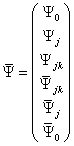
under chirality

where

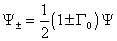
X_± = (1/2) (1 ± [capital gamma]₀) [psi]

and

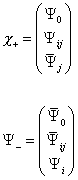
Therefore, for n = 5, [Psi bar]_i is the [5 bar]-dimensional representation. Ψ_ij is the 10-dimensional representation, and Ψ₀ is a singlet. All the fermions are assigned to Ψ₊.

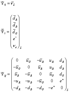
so there are the 16 particle states of SO(10) which are all in the Ψ₊ group.

The existence of the right-handed neutrino allows for the neutrinos to acquire mass in a similar way to the other fermions. However, you then have to explain why the neutrino masses are so much smaller than the other fermion masses. A possible explanation suggested by Gell-Mann, Ramond, and Slansky is to use the 126-dimensional representation of SO(10). Their idea was to give a nonzero vacuum expectation value to the SU(5) singlet part of the 126-dimensional representation of SO(10).

126 -> 1 + 5 + 10 + [10 bar] + 50 + [50 bar]

The Higgs representation that acquires vacuum expectation values in this case is the right-handed triplet, as in the left-right symmetric model. Therefore, the smallness of the neutrino mass is due to the suppression of V + A currents. You know how in the Standard Model, the weak force has a V – A current? This assumes the neutrino is massless. If the neutrino has mass, then there would also be V + A currents. However, if those currents are suppressed, that would explain why the neutrino masses are so small.

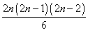
For SO(2n), the Higgs field φ_u is 2ⁿ dimensional, and the Higgs field φ_uvλ has a dimension of

(2n(2n – 1)(2n – 2)/6)

so for n = 5, φ_u is 10-dimensional, and φ_uvλ is 120-dimensional. The SU(5) singlet component of φ_uvλ has the form

X₁^† X₂^† X₃^† X₄^† X₅^†

or

X₁ X₂ X₃ X₄ X₅

This gives a Majorana mass only to the right-handed neutrino, while the Dirac masses arise from the introduction of the 10-dimensional Higgs. In the left-right symmetric model and SO(10), the neutrino masses are in the following matrix.

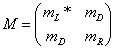
In a Dirac neutrino, m_L is equal to m_R = 0, and m_D is not zero.

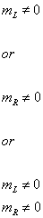
In a Majorana neutrino, either m_L or m_R, or both are nonzero. m_D is arbitrary.

In a Pseudo-Dirac neutrino, m_D is not zero. m_L is equal to m_R, and they are much less than m_D

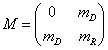
Working with chiral spinors, you choose the appropriate Higgs boson couplings so the mass matrix has the following form

In a more realistic model, minimization of the potential leads to the following modification of the mass matrix

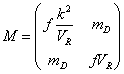
where V_R is the right-handed component of the Higgs potential, and k is a constant. This upsets the seesaw mechanism. This problem can be solved by breaking the D-parity present in SO(10), at the GUT scale separately from the SU(2)_R symmetry, by introducing a 210-dimensional or 45-dimensional Higgs multiplet. In this case, fk²/V_R

is replaced by fk²V_R/M_GUT²

which is tiny if M_GUT is large.

Since SO(10) contains the left-right symmetric model, it has an extra neutral Z⁰ boson called Z’. However, unlike the left-right symmetric model, the constraints of grand unification relate both g₁ and g₂ at the grand unification scale. Therefore, you have a specific symmetry breaking scheme, and the spectrum of the Higgs boson. All neutral current couplings at low energies are predicted in terms of the SU(2)_L gauge group. For SO(10), the neutral current Lagrangian is

L_{N. C.} = eQ_em A + g_uQ_ZZ + g_u Q_X Z_X

where in terms of SO(10) generators, you have

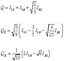
Q = I_3L + I_3R + [square root of 2/3] I_BL

Q_Z = [square root of 5/9] (I_3L = (3/5) I_3R – [square root of 6/25] I_BL)

Q_X = 1/[square root of 10] (27 I_3R – [square root of 6] I_BL)

where A is the photon field, and e = [square root of 3/8]g_u.

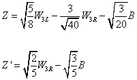
Z = [square root of 5/8] W_3L – (3/[square root of 40]) W_3R – [square root of 3/20] B

Z’ = [square root of 2/5] W_3R – [square root of 3/5] B

SU(5) and SO(10) are the two main grand unified theories, although there are others. There are grand unified theories based on the exceptional group E₆. There is an unusual grand unified theory called horizontal symmetry that attempts to explain why we have three generations of fermions. The Pati-Salam model is based on the group SU(4) x SU(2) x SU(2). The trinification model is based on the group [SU(3)]³ = SU(3) x SU(3) x SU(3). The 331 model is based on the group SU(3) x SU(3) x U(1).

One of the unanswered questions in physics is why is the Universe overwhelmingly composed of matter instead of antimatter. If there were large amounts of antimatter in the Universe, we would be able to detect a diffuse gamma ray background resulting from matter-antimatter annihilations. However, according to particle physics, particles should not be favored over antiparticles. If the Universe started out with equal amounts of matter and antimatter, it would not be able to get to the current overwhelming preponderance of matter over antimatter. Therefore, we have to explain the current matter-antimatter asymmetry. Since, a proton has a baryon number of 1, and an antiproton has a baryon number of -1, you could call this baryon asymmetry. Why does the Universe have a net positive baryon number?

Andrei Sakharov determined the three conditions, called the Sakharov criteria, that must be met to create the current baryon asymmetry.

1. B violation – Obviously, you need some way of violating baryon number in the first place.

2. C and CP violation – If C or CP are exact symmetries, then the total rate for any process that produces an excess of baryons is equal to the rate of the complementary reverse process that produces an excess of antibaryons, so no net baryon number is created.

3. Departure from thermal equilibrium.

Since grand unified theories, by their very nature, violate baryon number conservation, they are an obvious solution to the baryon asymmetry of the Universe. Unfortunately, even though they violate baryon number, they do not violate B – L. Even SO(10), which has a singlet associated with the antineutrino, which has a lepton number of -1, does not violate B – L. This choice of lepton number assignment does not lead to a new gauge boson that violates B – L. If B – L is conserved, then SO(10) is C symmetric. The generation of baryon asymmetry requires C violation. The C symmetry must be broken before baryon number can be created. However, the C symmetry is not broken until the U(1)_{B – L} symmetry is broken, at which time, it can’t violate baryon number, or such processes are very rare. Thus, grand unified theories, in their simple form, can’t explain the baryon asymmetry of the Universe. However, if you have an SO(10) model with a heavy Majorana neutrino to explain the smallness the light neutrino masses, then the decay of the right-handed neutrino can break B – L symmetry. This then does allow the possibility that grand unified theory could explain the baryon asymmetry.

To understand grand unification at a deeper level, you have to know more group theory than I’ve previously described. Unfortunately, this branch of mathematics is a vast and complicated subject, and an in depth comprehensive discussion of it would take us too far away from particle physics. Therefore, I will just briefly describe the main groups within the context of Dynkin diagrams. A Coxeter matrix of rank n is an n x n matrix M with M_ii = 1 and M_ij = M_ji > 1, and possibly infinite, for all i and j in (1, 2, … n). A Coxeter group is a group generated by the elements P_i with i in (1, 2, …n) subject to the relations

(P_i, P_j)^M_ij = 1

where M_ij are the elements of a Coxeter matrix.

A Coxeter diagram is a diagram used to visualize a Coxeter group. It is a labeled graph with nodes indexed by the generation of a Coxeter group, and (P_i, P_j) is an edge whenever M_ij > 2 which is labeled with M_ij, where M_ij is an entry in the Coxeter matrix corresponding to a given Coxeter group.

You can also talk about this in terms of taking reflections of vectors. Every element of a finite reflection group is a product of reflections through vectors called roots. These roots are all at angles π/n from each other, where n > 1 is an integer. To describe the group, you draw a diagram with one dot for each root. If two roots are perpendicular, you don’t draw a line between them. If they are at an angle π/n from each other, you draw one or more lines between them. If n = 3, you just draw one line. If n = 4, you draw two lines. If n = 5, you draw three lines. If n > 5, you draw one line, and label it with the integer n. Usually, the roots are all the same length, but if two roots are connected where one is shorter than the other, the line between them is marked with an arrow pointing to the shorter root. If the roots are the same length, that’s called simply laced. Here are the Coxeter diagrams for the finite reflection groups.

1.A_n, n > 0

A_n has a finite number of n dots. A₂ is the group of symmetries of an equilateral triangle. A₃ is the group of symmetries of a tetrahedron. More generally, A_n is the group of symmetries of an n-dimensional simplex, which are analogs of the tetrahedron in n dimensions.

The Lie algebra of A_n is sl_{{n + 1}} (c), the (n + 1) x (n – 1) complex matrices with vanishing trace, which form a Lie algebra. The compact real form of sl_{{n + 1}} (c) is su_n, and the corresponding compact Lie group is SU(n), the n x n unitary matrices of determinant 1. The symmetry group of the electroweak is U(1) x SU(2), where U(1) is the 1 x 1 unitary matrix. The symmetry group of the strong force is SU(3). The simplest grand unified theory has the symmetry group SU(5).

2.B_n, n > 1

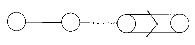
B_n has a finite number of n dots. The angle between the roots is π/4, so one of the edges has n = 4, which is represented by a double line. For B_n, all the roots except the last one are [square root of 2] times as long as the last one. Therefore, the arrow points to the last dot. B₂ is the group of symmetries of a square. B₃ is the group of symmetries of the cube or octahedron. More generally, B_n is the group of symmetries of an n-dimensional hypercube or hyperoctahedron in n dimensions.

The Lie algebra of B_n is so_{{2n + 1}} (C), the (2n + 1) x (2n + 1) skew-symmetric complex matrices with vanishing trace. The compact real form of SO_n (C) is so_n, and the corresponding compact Lie group is SO(n), the n x n real orthogonal matrices with determinant 1, which is the rotation group in Euclidean n-space. One of the main grand unified theories is based on SO(10). In superstring theory, you see the group SO(32).

3.C_n, n > 2

C_n is the same as B_n except that all the roots except the last one are 1/[square root of 2] times as long as the last one. Therefore, the last root is longer than the others, and the arrow points away from the last one to the others. Obviously, if there are just two roots, B_n and C_n are identical, and so to avoid redundancy, we say that for C_n, n > 2. B_n and C_n are duals to each other. C_n is also the group of symmetries of a hypercube or hyperoctahedron in n dimensions.

The Lie algebra for C_n is sp_n (C), the 2n x 2n complex matrices of the form

where B and C are symmetric, and D is minus the transpose of A. The compact real form of sp_n is sp_n, and the corresponding Lie group is called Sp(n). This is the group of n x n quaternionic matrices which preserve the usual inner product on the space Hⁿ of the n-tuples of quaternions.

4.D_n, n > 3

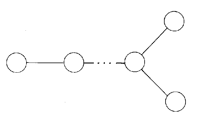
The Lie algebra of D_n is so_{2n} (C), the 2n x 2n skew-symmetric complex matrices with vanishing trace.

In unfortunate conflicting notation, sometimes you see D_n used to refer to the dihedral group which we’re calling I_m.

5.E₆

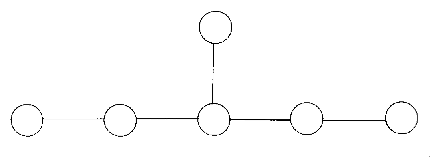
E₆ is a 78-dimensional Lie algebra. It’s smallest representation is 27-dimensional, consisting of all the 3 x 3 hermitian matrices over the octonions, on which it preserves the commutator. E₆ is used in grand unified theories. The E₆ group is important in the symmetry breaking of Heterotic E₈ x E₈ superstring theory.

6.E₇

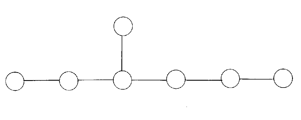
E₇ is a 133-dimensional Lie algebra. It’s smallest representation is 56-dimensional, on which it preserves a tetralinear form.

7.E₈

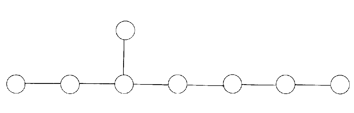
E₈ is a 248-dimensional Lie algebra, the biggest of the exceptional Lie algebras. It’s smallest representation is 248-dimensional, the adjoint representation in which it acts on itself. The easiest way to understand the Lie group E₈ is as the symmetries of itself. You can get its root lattice, the 8-dimensional lattice spanned by its roots, by using the icosahedron and quaternions. The E₈ group is used in superstring theory. Specifically, it appears in Heterotic E₈ x E₈ superstring theory.

8.F₄

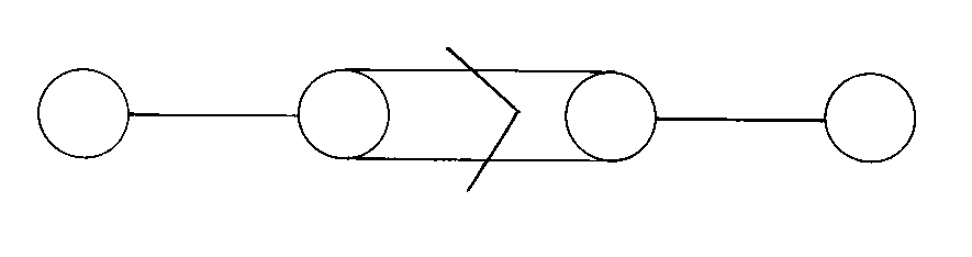
F₄ is a 52-dimensional Lie algebra. It’s smallest representation is 26-dimensional, consisting of traceless 3 x 3 hermitian matrices over the octonions, on which it preserves a trilinear form. F₄ is the group of symmetries of a four-dimensional polyhedron, or polytope, called the 24-cell. A four-dimensional polytope is called a polychoron.

9.G₂

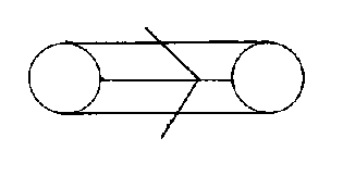
G₂ is a 14-dimensional Lie algebra, and the compact Lie group corresponding to its compact real form is also called G₂. This group is the group of symmetries, or automorphisms, of the octonions. The smallest representation of this Lie algebra is 7-dimensional, corresponding to the purely imaginary octonions. The G₂ group is relevant to the type of manifold that is used to compactify the extra dimensions in M-theory.

10.H₃

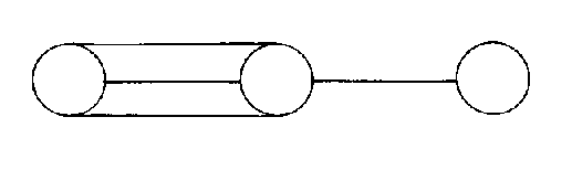
H₃ is the group of symmetries of the dodecahedron and icosahedron. There is no associated Lie algebra.

11.H₄

H₄ is the group of symmetries of a four dimensional polyhedron, or polytope, called the unit icosian or 120-cell, which has 120 vertices, and is closely related to the dodecahedron and iscosahedron. There is no associated Lie algebra. The fact that the H groups stop at four is the reason why there are no analogs of the dodecahedron or icosahedron in more than four spatial dimensions.

12.I_m, m = 5 or m > 6

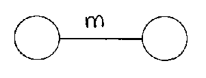
I_m corresponds to the symmetry group of the 2m-gon, or polygon with 2m sides, in a plane. There is no associated Lie algebra.

A lattice is formed by taking n linearly independent vectors in n-dimensional Euclidean space, and forming all possible linear combinations with integer coefficients. Whether or not there exists a lattice for a given symmetry group is called the crystallographic condition. If a symmetry group satisfies the crystallographic condition, then there exists a symmetry group with that symmetry. In the above list, the ones that satisfy the crystallographic condition are

A_n, B_n, C_n, D_n, E₆, E₇, E₈, F₄, and G₂

These are the symmetry groups corresponding to the semisimple Lie algebras of the same name. Their Coxeter diagrams are called Dynkin diagrams. There are four infinite groups, called the classical series, and five others, called the exceptional groups. The fact that the H groups do not satisfy the crystallographic condition is the reason why there are no naturally occurring crystals with dodecahedral or icosahedral symmetry, although in 1982, Dan Shechtman discovered quasicrystals, which can have dodecahedral or icosahedral symmetry. Dan Shechtman received the 2011 Nobel Prize in Chemistry for the discovery of quasicrystals.

If you take a d-dimensional polytope, such as a regular polygon or polyhedron, and you exchange the (d – 1)-dimensional components with vertices, and vice versa, you get a dual to the original polytope. For example, the dual of the cube is the octahedron. If the polytope is associated with a Dynkin diagram that has left-right symmetry, then the polytope is self-dual.

The infinite series of simple Lie groups associated to rotations in real vector spaces which are the SO(n) groups, are the B and D series. The infinite series of simple Lie groups associated to rotations in complex vector spaces is the SU(n) groups, which is the A series. The infinite series of simple Lie groups associated to rotations in quaternionic vector spaces is the Sp(n) groups, which is the C series. The five exceptional groups are related to the octonions.

Now let’s try taking the Dynkin diagram of the biggest exceptional Lie algebra, and keep removing the right most dot, and see what happens. You start with E₈.

This group is important in superstring theory. Now remove the right most dot, and you get E₇.

Now do the same thing again, and you get E₆.

E₆ is used in grand unified theories. Remove the right most dot again.

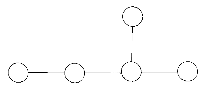
This is SO(10) which is used in grand unified theories. Remove the right most dot again.

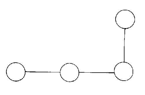
This is SU(5) from grand unified theory. Now remove the right most dot from the line of dots we were removing them from.

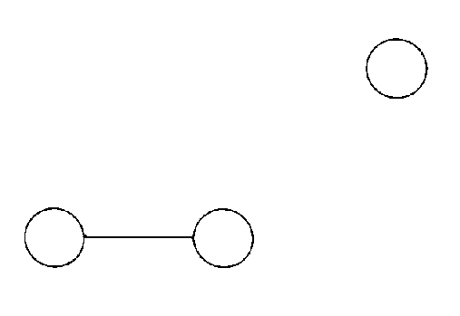
This is the SU(3) x SU(2) group of the Standard Model. Notice that just by repeatedly removing the right most dot, we continually get groups that are important in particle physics. First E₈, then E₆, SO(10), SU(5), and the Standard Model. You take the largest possible exceptional group, and repeatedly remove the right most dot, and you will get only groups important in particle physics, except for E₇, and you will get all the groups important in particle physics, except for SO(32). This has to do with the fact that in grand unified theory, the groups are nestled within each other, and each group is contained in a larger group. As you go through symmetry breaking, you go from larger to smaller groups.

The quarks and leptons can be united in grand unified theories. However, a more ambitious goal is to unite the two broadest categories of particles, which are the fermions and bosons. This is called supersymmetry, or SUSY. There are several reasons for supporting supersymmetry beyond the aesthetic appeal of unifying the fermions and bosons. Most important is the problem of quadratic divergences, which are contributions to the mass of the Higgs particle, which drive up the Higgs mass to unacceptable levels, violating the unitarity condition. This is called the hierarchy problem. In supersymmetry, contributions from both fermions and bosons cancel out, leaving a much smaller Higgs mass, thereby solving the hierarchy problem. In grand unified theories, the coupling constants almost converge but not quite. In supersymmetry, they exactly converge. In an extension of supersymmetry called supergravity, there is a natural way of including gravity, although it doesn’t solve the problem of renormalization. Lastly, the lightest supersymmetric particle should be stable, and is thus a candidate for dark matter.

In supersymmetry, every fermion is associated with a boson that’s name is the same except begins with “s-“, and with a spin that is ½ less. Every boson is associated with a fermion that’s name is the same except ends with “-ino”, and with a spin that is ½ less. Therefore, the electron is associated with the selectron, which has spin 0. The photon is associated with the photino, which has spin ½. The other quantum numbers are the same. Supersymmetric particles are represented by a tilda over the letter.

Supersymmetry was invented independently by several people with different motivations. In 1971, Soviet physicists Yuri Gol’fand and E. Lictman came up with an early theory while trying to introduce parity violation into quantum theory. In 1972, Volkov and Akulov were trying to answer the question as to whether Goldstone bosons with half spin exist. However, most people agree that the main inventors of supersymmetry were Julius Wess and Bruno Zumino in 1974, who were performing a generalization of the subgroup which first appeared in the Neveu-Schwarz-Ramond model, thereby discovering quantum field theories with spacetime supersymmetry in four spacetime dimensions.

Let’s look at the hierarchy problem in more detail since it is the main motivation for supersymmetry. A phenomenological field theory such as the Standard Model must be cut off at small distances to be defined. The formal path integral is meaningless until a prescription is given for regularizing its short distance behavior. This prescription specifies a momentum k as a cut off, and a set of parameters including coupling constants g, and a mass parameter u, which will generally depend on k. Of course, there exist quantum fluctuations less than the wavelength but the whole point of renormalization is that these effects can be lumped into the various values of the constants g and u. A change in the cutoff from k to k’ can be compensated by a change in g and u. In this way, the Standard Model can deal with changes to the parameters that result from virtual particles constantly be emitted and reabsorbed by bosons and fermions, but not the Higgs particle. The mass of the Higgs would be driven up to unacceptable levels. This is because the Higgs two-point function contains not just logarithmic but also quadratic divergences. This causes the Higgs mass to be so high that it violates unitarity. This is the hierarchy problem. What actually causes these corrections to the masses of the particles? The measured electron mass is a combination and the bare mass and the self-energy, which is the result of the electron emitting and reabsorbing virtual photons. Therefore, the correction to the mass is caused by the self-energy which is caused by the loop diagrams of virtual particles. However, the loop diagrams of virtual fermions and bosons have the opposite effect. In supersymmetry, there’s a boson for every fermion, and vice versa, so these loop diagrams cancel each other out, so you don’t have the very large correction term for the Higgs mass.

In my paper on the Standard Model, I skipped over some of the details of quantum field theory, so let me just briefly review them. In quantum field theory, you want the wavefunction of a particle to only propagate forward and not backwards in time. You use Green’s function to distinguish between the two arrows of time. If you have a scalar field wave equation with a delta function source

([D’Alambertian] + m²) G = -[delta]⁽⁴⁾ (x^u – x’^u)

the Green function G(x^u, x’^u) that solves this equation is found by going to momentum space, where

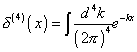
[delta]⁽⁴⁾ = [integral] (d⁴/(2[pi])⁴) e^-ikx

This gives the Feynman propagator

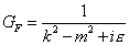
G_F = 1/(k² – m² + i[epsilon])

where k is momentum, m is mass, and the small positive ε is set to zero after performing momentum space integrations. This then gives you the propagator for the scalar field

<0|T[[phi](x) [phi](x’)]|0> = i[integral] (d⁴/(2[pi])⁴) e^{-ik(x – x’)}(1/(k² – m² + i[epsilon]))

Let’s first look at the case of the photon self-energy taking into account the one-loop correction to the Feynman diagram. The photon becomes an electron-positron pair which then turns back into a photon. These examples will be two-point functions, since there are two vertices, at vanishing momentum, computed at one-loop level. The computed quantities correspond to the mass parameters appearing in the Lagrangian, and since we assume vanishing external momentum, this will not be the on-shell pole mass. It is easy to see that the differences between these two quantities can at most involve logarithmic divergences due to wave function normalization. The following shows the photon self-energy in QED.

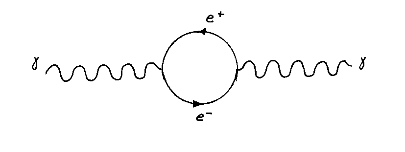
The following is the photon’s two-point function which receives contributions due to the electron-positron loop diagram.

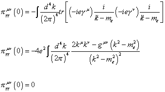
[pi]_{[gamma] [gamma]}^uv (0) = -[integral] (d⁴k/(2[pi])⁴) tr[(-ie[gamma]⁴) (i/[k slash] -m_e) (-ie[gamma]^u) (i/([k slash] – m_e))

[pi]_{[gamma] [gamma]}^uv (0) = -4e² [integral] (d⁴k/(2[pi])⁴) ((2k^u k^v – g^uv (k² – m_e²))/(k² – m_e²)²)

[pi]_{[gamma] [gamma]}^uv (0) = 0

The integral vanishes because of the regularization scheme that preserves gauge invariance, called dimensional regularization. At a deeper level, it’s because of the exact U(1) gauge invariance of QED, which says that the photon must be massless in all orders of perturbation theory.

The following shows the electron self-energy in QED.

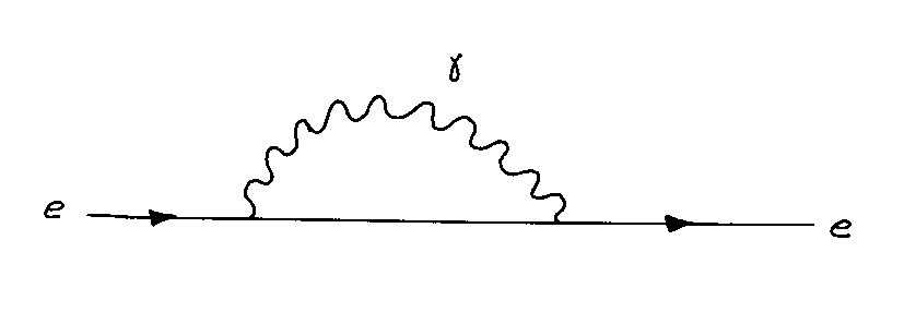
The electron self-energy correction is given by

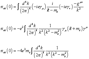
[pi]_ee (0) = [integral] (d⁴k/(2[pi])⁴)b(-ie[gamma]_u) (i/[k slash] – m_e) (-ie[gamma]_u) (-ig^uv/k²)

[pi]_ee (0) = -e² [integral] (d⁴k/(2[pi])⁴) (1/(k²(k² – m_e²)) [gamma]_u ([k slash] + m_e) [gamma]^u

[pi]_ee (0) = -4e² m_e [integral] (d⁴k/(2[pi])⁴) (1/(k²(k² – m_e²))

using the fact that the ([k slash] – m_e) term vanishes after integration over angles, if you use a regulator that respects Poincare invariance. The integral in the above equation has a logarithmic divergence in the ultraviolet, meaning at large momenta. Notice that this correction to the electron mass is proportional to the electron mass. Without a cutoff, the correction is infinite, but if you use the Planck scale as the cutoff scale, the mass correction is

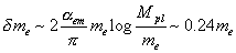
[delta]m_e ~ ([alpha]_em/[pi]) m_e (M_pl/m_e) ~ 0.24 m_e

which is a small correction. The reason the loop diagram doesn’t change the electron mass by much is due to symmetry. In the limit m_e -> 0, the model becomes invariant under chiral rotations.

[psi]_e -> e^{i[gamma]₅[psi]} [psi]_e

If the symmetry was exact, the mass correction would vanish. Since the symmetry is broken by the electron mass, the mass correction itself must be proportional to m_e.

Now, we’ll consider the contributions of fermion loops to the two-point function of the Standard Model Higgs field.

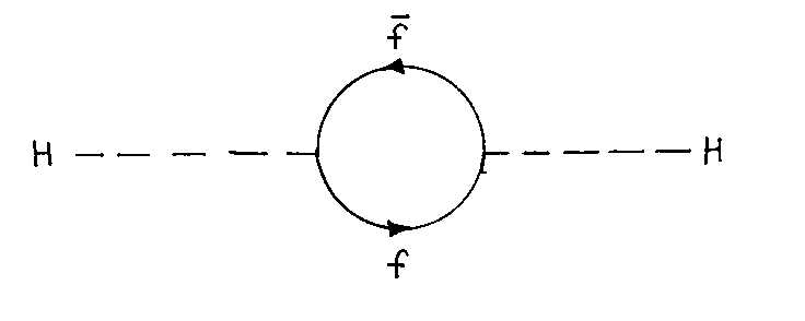
With the Hf[f bar] coupling given by the coupling constant [lambda]_f, the mass correction is given by

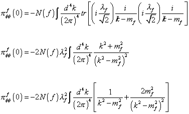
[pi]_{[phi] [phi]}^f (0) = -N(f) [integral] (d⁴k/(2[pi])⁴) tr [ (i([lambda]_f/[square root of 2]) (i/[k slash – m_f) (i[lambda]_f/[square root of 2]) (i/[k slash] – m_f)]

[pi]_{[phi] [phi]}^f (0) = -2N(f) [lambda]_f² [integral] (d⁴k/(2[pi])⁴) ((k² + m_f²)/(k² – m_f²)²)

[pi]_{[phi] [phi]}^f (0) = -2N(f) [lambda]_f² [integral] (d⁴k/(2[pi])⁴) [(1/(k² – m_f²)) + (2m_f²/(k² – m_f²)²)]

where the multiplicity factor N(f) is three for quarks, and one for leptons. The first term in the last line of the above equation is quadratically divergent. If you were to use the Planck mass as a cutoff, the resulting correction would be 30 times larger than the Standard Model Higgs mass, which is assumed to be about 1 TeV. If the Higgs mass is much larger than 1 TeV, it would violate the unitarity condition in regards to the WW scattering amplitudes. You can define unitarity as saying the probability of something can’t be greater than 1. U U^† = 1 If the Higgs mass is too big, Higgs self-interaction will make the coupling constant bigger than 1. Also, if m_H is too big, the decays H → W W and H → Z Z will have a full decay width as large as the Higgs mass. These are all considered impossible, so the Higgs mass can’t be larger than about 1 TeV.

The difference in the size of the mass correction to the electron and the Higgs illustrates the difference between logarithmic and quadratic divergences. Also notice that the correction does not depend on the mass of the Higgs. There is nothing in the Standard Model that protects the mass of the Higgs in the way that the photon and electron masses are protected.

Now you can renormalize the quadratic divergence away. The remaining correction would be of order

N(f) ((m_f² [lambda]_f²)/8[pi])

If the Standard Model were the ultimate theory in physics, and m_f were the mass of the top quark, then the correction would be small. However, nobody thinks the Standard Model is the final theory in physics. It is much more plausible that at some very high energy scale, it will have to be replaced with a more fundamental theory, such as grand unification. In a grand unified theory, m_f would be at the GUT scale, which would cause the correction to be extremely large. Even without grand unification, there is probably new physics at the Planck scale. Now, you can still assume a very large bare mass to cancel out the very large loop corrections, leaving a result of about 1 TeV. However, in that case, you would have to assume the coincidence that these two very large values were so close as to almost cancel out. This is called a fine-tuning problem, which you want to avoid in physics. Let’s assume u² (0) has the form

u² (0) = u² (k) + k² (c₁ [lambda] + c₂ g² + …)

Let’s assume the cutoff k is at the energy of the GUT scale.

u² (0) = u² (M_GUT) + M_GUT² (c₁ [lambda] (M_GUT) + …)

If M_GUT = 10¹⁵ GeV, this gives

((u² (0))/M_GUT²) = ((u² (M_GUT))/(M_GUT²)) + (c₁ [lambda] + …) = 10^-26

This would require the dimensionless parameter to cancel out the complicated series to 26 decimal places. In other words, this would require enormous fine-tuning which does not seem realistic.

In supersymmetry, you assume that for every fermion, there is an associated boson. You have to take into account the one-loop diagrams of both the fermions and bosons when calculating the correction to the Higgs mass. As it turns out, the effects from these two types of loop diagrams cancel out.

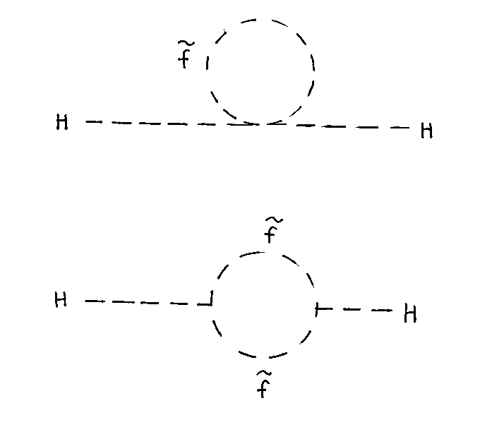
Let’s say you have two complex scalar fields [f tilda]_L and [f tilda]_R with the following coupling to the Higgs field

L_{[phi] [f tilda]} = (1/2) [lambda tilda]_{f [phi]} ( | [f tilda]_L |² + | [f tilda]_R |² ) + v[lambda tilda]_f [phi] ( | [f tilda]_L |² + | [f tilda]_R |² ) + (([lambda]_f/[square root of 2) A_f [phi] [f tilda]_L [f tilda]_R* + hermitian conjugate

where v is the vacuum expectation value of the Standard Model Higgs. v = 246 GeV The second term in the Lagrangian is due to the breaking of the SU(2) x U(1), and its coefficient is related to that of the first term. The coefficient of the third term is arbitrary. λ_f is a convention. This Lagrangian gives the following contribution.

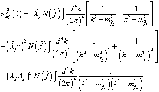
[pi] _{[phi] [phi]}^{[f tilda]} (0) = -[lambda tilda]_f N(f) [integral] (d⁴k/(2[pi])⁴) [(1/(k² – m_{[f tilda]L}²)) + [(1/(k² – m_{[f tilda]R}²))] + ([lambda tilda]_f v)² N([f tilda]) [integral] (d⁴k/(2[pi])⁴) >) [(1/(k² – m_{[f tilda]L}²)²) + [(1/(k² – m_{[f tilda]R}²)²)] + | [lambda]_f A_f |² N([f tilda]) [integral] (d⁴k/(2[pi])⁴) (1/((k² – m_{[f tilda]L}²)(k² – m_{[f tilda]R}²))

The first line comes from the first loop diagram, and contains quadratically divergent terms. The quadratic divergences can be made to cancel by choosing

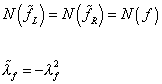
N([f tilda]_L) = N([f tilda]_R) = N(f)

[lambda tilda]_f = -[lambda tilda]_f²

The cancellation of divergences does not impose restrictions on the masses, m_{[f tilda]L}, m_{[f tilda]R}, or the coupling constant A_f

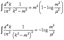
[integral] (d²/i[pi]²) (1/(k² – m²)) = m² (1 – log (m²/u²))

[integral] (d²/i[pi]²) (1/(k² – m²)²) = – log (m²/u²))

where u is the renormalization scale. For simplicity, let’s assume , m_{[f tilda]L} = m_{[f tilda]R} = m_{[f tilda]}. This gives

[pi]_{[phi] [phi]}^{f + [f tilda]} = i(([lambda]_f² N(f))/(16[pi]²)) [-2m_f² (1 – log (m_f²/u²)) + 4m_f² log (m_f²/u²) + 2m_{[f tilda]}² (1 + log (m_f²/u²) + 2m_{[f tilda]}² (1 + log (m_{[f tilda]}²)) – 4m_f² log (m_{[f tilda]}²) – | A_f|² (m_{[f tilda]}²)]

using

m_f = ([lambda]_f v)/[square root of 2]

The first two terms are the fermionic contribution. Therefore, you achieve complete cancellation between the fermionic and bosonic contributions. You achieve a vanishing total correction if you require

m_{[f tilda]} = m_f

A_f = 0

Even if you let m_f go to infinity, the correction will remain small as long as the difference between m_f² and m_{[f tilda]}² remains small, and the coefficient A_f remains small. Therefore, the introduction of the fields [f tilda]_L and [f tilda]_R has not only allowed us to cancel quadratic divergences, but it also shields the weak scale from loop corrections involving heavy particles if the mass splitting between the fermions and bosons itself is at the weak scale. Therefore, supersymmetry solves the hierarchy problem.

I should also mention an alternative explanation for the hierarchy problem called technicolor. This used to be a serious rival to supersymmetry, but it does not work near as well, and so far no one has come up with a version of it that doesn’t contradict reality. Still, in order to be knowledgeable about physics beyond the Standard Model, you should be aware of what technicolor is. In a way, technicolor is more accurately described as an alternative to the Higgs mechanism, but of course if there’s no Higgs particle, then there’s no hierarchy problem. The Higgs mechanism is a way of giving masses to the W⁺, W^–, and Z⁰ bosons. Through the breaking of a global symmetry, the associated goldstone boson becomes the longitudinal component of the W⁺, W^–, and Z⁰ bosons, thereby giving them mass. There are, of course, other examples of spontaneous symmetry breaking, one of which is the chiral symmetry of QCD. In that case, the associated goldstone boson is assumed to be the neutral pion. Could you use the symmetry breaking of the QCD chiral symmetry, SU(2) x U(1), to give mass to the W⁺, W^–, and Z⁰ bosons? Yes, that is possible. The chiral multiplet is isomorphic to the Higgs multiplet. The pion multiplet would mix with the gauge fields, and become the longitudinal component of the W⁺, W^–, and Z⁰. There would be no Higgs particle, and thus no hierarchy problem.

The problem is that the masses of the resulting W⁺, W^–, and Z⁰ would be 2000 times too small. However, let’s say you invented a second QCD-like gauge sector called technicolor. This gauge group does not have to be SU(3), and it should become strong at 2000 times the QCD scale. If this sector contains fermions which carry technicolor instead of color, but which form conventional weak doublets, then condensates will induce SU(2) x U(1) breaking. The W⁺, W^–, and Z⁰ will get masses of the correct magnitude, and no very small or fine-tuned parameters are needed. The main prediction of technicolor is the prediction of a spectrum of technihadrons with masses, widths, and splittings 2000 times their hadronic counterparts. So far so good. Unfortunately, there is a serious problem with technicolor which no one has been able to satisfactorily solve, namely that there is no mechanism to give masses to the fermions. Remember that in the Standard Model, the fermion-Higgs interaction terms allow for fermion masses. However, in technicolor, there are no Higgs particles, so you can’t do that, and so you have to think of some other way of giving mass to the fermions. One idea called extended technicolor introduces new gauge degrees of freedom, called E, which couple ordinary fermions to technifermions. This ends up giving mass to the fermions. Another idea is that quarks, leptons, and technifermions are all composites of more fundamental particles called preons, bound by yet a third strong interaction called metacolor. The binding energy can give mass to these composite particles. However, all of these ideas conflict with observation in one way or another, for instance, in the prediction of neutral strangeness changing currents, etc. Therefore, technicolor just doesn’t seem to work, and supersymmetry won that debate.

In quantum mechanics, energy is quantized, meaning you have discrete energy levels associated with particles.

H_N = [summation over i] N_j [epsilon]_j

where H_N is the Hamiltonian, and N_j is the number of particles in each energy state. Therefore

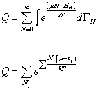
Q = [summation over N] [integral] e^{((u N – H_N)/kT)} d[capital gamma]_N

Q = [summation over N_j] e^{[summation N_j (u – [epsilon]_j)/kT}

where k is the Boltzmann constant, k = 1.38066 x 10^-23 J/K, and T is the temperature. Then using

e^{[summation] x_j} = [product series over j] e^x_j

you have

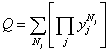
Q = [summation over N_j] [[product series over j] y_j^N_j]

where

y_j = e^{((u – [epsilon]_j)/kT)}

using

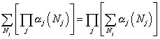
[summation over N_j] [[pi] [alpha]_j (N_j)] = [product series over j] [[summation over N_j] [alpha]_j (N_j)]

you end up with

Q = [product series over j] [summation over N_j] y_j^N_j

The following power series has the following convergent sum

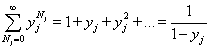
[summation over N_j from 0 to infinity] y_j^N_j = 1 + y_j + y_j² + … = 1/(1 + y_j)

so

Q = [product series over j] 1/(1 – y_j)

Therefore

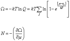
[capital omega] = -k + ln Q = k + [summation over j] ln [1 – e^{(u – [epsilon]_j)/kT}]

N = – [partial derivative of capital omega with respect to u]

where Ω is the grand potential.

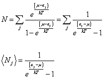
N = [summation] (e^{(u – [epsilon]_j)/kT})/(1 – e^{(u – [epsilon]_j)/kT}) = [summation] 1/( e^{(( [epsilon]_j – u)/kT}) – 1)

N_j = 1/( e^{(([epsilon]_j – u )/kT}) – 1)

This is the average occupation number if you can have any number of particles in a single state, meaning not obey the Pauli exclusion principle, in other words, bosons. What if you can have only zero or one particle in each state, meaning particles that obey the Pauli exclusion principle, or in other words, fermions?

Before we considered the possibility that you could have an arbitrary number of particles in any given energy state, and therefore took a summation of every value of N_j from zero to infinity. Now, let’s assume N_j can only take two values, zero or one, meaning you only have either zero or one particles in each energy state. If N_j = 0 or 1, then

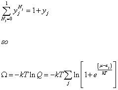
[summation over N_j from 0 to 1] y_j^N_j = 1 + y_j

so therefore

[capital omega] = -k + ln Q = -kT [summation] ln [1 + e^{((u – [epsilon]_j)/kT)}]

with

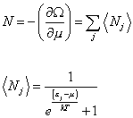
N = -[partial derivative of capital omega with respect to u] = [summation] (N_j)

N_j = 1/( e^{(([epsilon] – u )/kT}) + 1)

The above results for bosons and fermions are called the statistics, and give the statistical rules which apply to large numbers of particles. Bosons obey Bose statistics, also called Bose-Einstein statistics, partly named after Satyendra Nath Bose. Fermions obey Fermi statistics, also called Fermi-Dirac statistics, named after Enrico Fermi and Paul Dirac. Notice the above result for fermions is exactly the same result as for bosons except there is a plus sign instead of a minus sign. The Bose statistics have a minus sign, and the Fermi statistics have a plus sign. This is the ultimate reason why the algebra of bosons involves commutators, and the algebra of fermions involves anticommutators. Remember that a commutator is defined as

[a, b] = ab – ba

and an anticommutator is defined as

{a, b} = ab + ba

For normal numbers, [a, b] = 0. However, the only normal number for which {a, b} = 0 is zero. Therefore, we invented entities called Grassmann variables which satisfy {a, b} = 0.

Remember in the electromagnetism section of my paper on the Standard Model, I gave the following relations for the energy of a particle system.

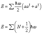
E = [summation] ([h bar]w/2) (a a^† + a^† a)

E = [summation] (N + (1/2)) [h bar]w

where [a, a^†] = 1, and the number operator N = a^† a. Notice the energy is nonzero even if N = 0. Therefore, you have vacuum energy. This is a bosonic field since we quantized via the commutator [a, a^†] = 1. In supersymmetry, every bosonic field is matched by a corresponding fermionic field. The fermionic fields would be quantized via the anticommutator {a, a^†} = 1, which gives

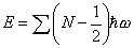
E = (N – (1/2)) [h bar]w

Therefore, when the total number of particles is zero, N = 0, the bosonic part gives

E = (1/2)[h bar]w

and the fermionic part gives

E = – (1/2)[h bar]w

and so they cancel each other out exactly. Therefore, if supersymmetry were unbroken, you would have zero vacuum energy. Even though it’s not unbroken at low energies, they cancel out at high energies where supersymmetry is unbroken. Therefore, above the supersymmetry breaking scale, the bosonic and fermionic contributions to the Higgs mass cancel out. Supersymmetry adds fermionic contributions along with the bosonic contributions to the self-energy of the Higgs mass to solve the hierarchy problem.

The fermionic and bosonic contributions to the vacuum energy also cancel out. If there was an unbroken supersymmetry, we would have no vacuum energy, although obviously we don’t have an unbroken supersymmetry. However, the fermionic and bosonic contributions to the vacuum energy will cancel out above the supersymmetry breaking scale. Therefore, supersymmetric models predict a vacuum energy only 10⁵⁵ times larger than the observed value, instead of 10¹²⁰ times larger.

Therefore, what supersymmetry ultimately boils down to is including anticommutators along with commutators. A symmetry of the S-matrix means that symmetry transformations have the effects of merely reshuffling the asymptotic single and multiparticle states. The Coleman-Mandula theorem, postulated by Sidney Coleman and Jeffrey Mandula in 1967, states that the only symmetries of the S-matrix are the following.

1. Poincare invariance, which is the semi-direct product of translated and Lorentz rotations, with generators P_m and M_mn.

2. Internal global symmetries, related to conserved quantum numbers, such as electric charge and isospin. The symmetry generators are Lorentz scalars, and generate a Lie algebra.

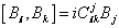
[B_l, B_k] = iC_lk^j B_j

where C_lk^j are structure constants.

3. Discrete symmetries, which are C, P, and T.

In 1975, Haag, Lopuszanski, and Sohnius proved that by weakening the assumptions of the Coleman-Mandula theorem, you end up with supersymmetry. Specifically, they weakened the assumption that the symmetry algebra of the S-matrix involves only commutators. If you allow both commutating and anticommutating generators, you end up with supersymmetry. Supersymmetry is the introduction of anticommuting symmetry generators which transform as the ( ½, 0) and (0, ½) spinor representations of the Lorentz group. Since these new symmetry generators are spinors, not scalars, supersymmetry is not an internal symmetry. Rather, it is an extension of the Poincare symmetry by anticommuting spinor generators.

The new symmetry we are looking for must connect bosons and fermions. In other words, the generators Q of this symmetry must turn a bosonic state into a fermionic state, and vice versa. This in turn implies that the generators themselves carry half-integer spin, and are thus fermionic. This is in contrast to the generators of the Lorentz group, or with gauge group generators, which are all bosonic. The simplest choice of SUSY generators is a 2-component Weyl spinor Q, and its conjugate [Q bar]. Since the generators are fermionic, their algebra can be most easily written in terms of anticommutators.

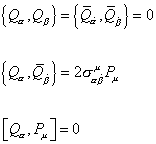
{Q_[alpha], Q_[beta]} = {[Q bar]_{[alpha dot]}, [Q bar]_{[beta dot]}} = 0

{Q_[alpha], [Q bar]_{[beta dot]}} = 2[sigma]_{[alpha] [beta dot]}^u P_u

[Q_[alpha], P_u] = 0

where α and β of Q, and [α dot] and [β dot] of [Q bar] take values 1 or 2. σ^u = (1, σ_i) where σ_i are the Pauli spin matrices. P_u is the translation generator. For a compact description of SUSY transformations, we introduce fermionic coordinates θ and [θ bar]. These are anticommuting Grassmann variables.

{[theta], [theta]} = {[theta], [theta bar]} = {[theta bar], [theta bar]} = 0

A finite SUSY transformation can be written as

e^{i([theta]Q + [Q bar] [theta bar] – x_u Pu)}

compared to a non-abelian gauge transformation

e^i[psi]_a Ta

where T^a is the group generators.

The objects on which SUSY transformations acts on must also depend on θ and [θ bar]. You therefore need superfields which are functions of θ and [θ bar] as well as the spacetime coordinates x_u. Since θ and [θ bar] are two component spinors, you could even say that supersymmetry doubles the dimensions of spacetime, the new dimensions being fermionic. Poincare transformations are transformations from one reference frame to another, and supersymmetry is an extension of that, so you could think of it as movement into some sort of superspace within which bosons and fermions exchange identities. I should emphasize that very few people think of supersymmetry in that way. Most people tend to think of it more like a discrete symmetry, such as turning a particle into its antiparticle, although mathematically it’s not. Thus, you have a discrepancy between how supersymmetry transformations are handled mathematically, and how they are handled psychologically.

For most practical purposes, it’s sufficient to consider infinitesimal SUSY transformations which are written as

[delta]_s([alpha], [alpha bar]) [capital phi] (x, [theta], [theta bar]) = [[alpha] [partial derivative with respect to theta] + [alpha bar] [partial derivative with respect to theta bar] – i([alpha] [sigma]_u [theta bar] – [theta] [sigma]_u [alpha bar]) [partial derivative with respect to x_u]] [capital phi] (x, [theta], [theta bar])

where Φ is a superfield, and α and [α bar] are Grassmann variables. This corresponds to the following explicit representation of the SUSY generators.

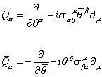
Q_[alpha] = [partial derivative with respect to [theta]^[alpha]] -i[sigma]_{[alpha] [beta dot]}^u [theta bar]^{[beta dot]} [partial derivative with respect to u]

[Q bar]_{[alpha dot]} = -[partial derivative with respect to [theta bar]^{[alpha dot]}] + i[theta]^[beta] [sigma]_{[beta] [alpha dot]}^u [partial derivative]_u

The following are the SUSY-covariant derivatives which anticommute with the SUSY transformations.

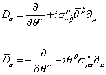
D_[alpha] = [partial derivative with respect to [theta]^[alpha]] + i[sigma]_{[alpha] [beta dot]}^u [theta bar]^{[beta dot]} [partial derivative with respect to u]

[D bar]_{[alpha dot]} = -[partial derivative with respect to [theta bar]^{[alpha dot]}] – i[theta]^[beta] [sigma]_{[beta] [alpha dot]}^u [partial derivative]_u

The above equations have been written in such a way as to treat θ and [θ bar] the same. It’s often convenient to use chiral representation where θ and [θ bar] are treated slightly differently.

Left-handed or L-representation

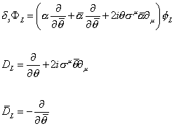
[delta]_s [phi]_L = ([alpha] [partial derivative with respect to [theta bar]] + [alpha bar] [partial derivative with respect to [theta bar]] + 2i[theta] [sigma]^u [alpha bar] [partial derivative]_u) [capital phi]_L

D_L = [partial derivative with respect to [theta]] + 2i[sigma]^u [theta bar] [partial derivative]_u

[D bar]_L = -[partial derivative with respect to [theta bar]]

Right-handed or R-representation

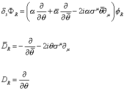
[delta]_s [capital phi]_R = ([alpha] [partial derivative with respect to [phi]] + [alpha bar] [partial derivative [theta bar]] – 2i[alpha] [sigma]^u [theta bar] [partial derivative]_u) [capital phi]_R

[D bar]_R = -[partial derivative with respect to [theta bar]] – 2i[theta] [sigma]^u [partial derivative]_u

D_R = [partial derivative with respect to [theta]]

Notice that [D bar] has a particularly simple form in the L-representation, and D has a particularly simple form in the R-representation. Normally, you choose the representation that would most simplify the notation. However, you have to stick with whichever representation you’re using, so you don’t always have the luxury of writing a given quantity in the representation that would give it the simplest form. The following identity allows you to go back and forth between representations.

[capital phi] (x, [theta], [theta bar]) = [phi]_L (x_u + i[theta] [sigma]_u [theta bar], [theta], [theta bar]) = [phi]_R (x_u -i[theta] [sigma]_u [theta bar], [theta], [theta bar])

So far, everything has been written for arbitrary superfields. However, at this point, you need to specify two special kinds of superfields called irreducible superfields. The two kinds of irreducible superfields are called chiral superfields and vector superfields.

The first type of superfield is the chiral superfield. The Standard Model fermions are chiral. Their left-handed and right-handed forms transform differently under SU(2) x U(1). This is another way of saying the weak force is parity violating. Therefore, you need superfields with two fermionic degrees of freedom, which can then describe the left-handed and right-handed components of the Standard Model fermions. Of course, the same superfields also contain bosonic partners, the sfermions. Therefore, you require either

[D bar] [phi]_L = 0

where φ_L is left chiral, or

D [phi]_R = 0

where φ_R is right chiral. Notice that these are very simply expressed using the chiral representation of SUSY generators, or SUSY-covariant derivatives. For instance, the L-representation, φ_L, is independent of [θ bar]. Remembering that θ is an anticommuting Grassmann variable, you can expand φ_L as

[capital phi]_L (x, [theta]) = [phi](x) + [square root of 2] [theta]^[alpha] [psi]_[alpha](x) + [theta]^[alpha] [theta]^[beta] [epsilon]_{[alpha] [beta]} F(x)

where summation over identical indices is assumed, and ε_{α β} is the Levi-Civita tensor. F is a scalar field. φ has dimensions of mass. θ has dimensions of mass^-½. The fermionic field has dimensions of m^-3/2. The superfield φ has dimensions of mass. So far, this is what you would expect. However, in order to be dimensionally consistent, the field F would have to have the unusual dimensions of m², which is hard to interpret. If something has dimensions of massⁿ, or mⁿ, you say it has mass dimension n. Another problem is that Φ_L seems to contain four bosonic degrees of freedom, and only two fermionic degrees of freedom, so they do not cancel.

However, these two puzzles in fact solve each other. The fact F has dimensions of m² means that a free kinetic term for F would be dimensionally inconsistent, which means it’s not a propagating field. Therefore, not at all of the bosonic fields represent physical propagating degrees of freedom. Therefore, there are equal numbers of propagating bosonic and fermionic degrees of freedom. As it turns out, F, and another field I’ll mention later called D, are auxiliary fields that have to be introduced partly because a fermion has more degrees of freedom than a boson. They are eventually eliminated. You could think of them purely as a book keeping device. You could also think of them as particles that exist only as internal lines in Feynman diagrams, and never appear in external lines. For instance, if you have a quadralinear Higgs vertex, meaning four Higgs lines meeting at a single vertex, you could imagine it as two trilinear Higgs vertices, where two Higgs particles exchange an F particle.

The result for φ_R in R-representation is the same as that for φ_L in L-representation, replacing θ with [θ bar]. You could, of course, write a left-handed superfield using right-chiral representation of the SUSY generators, or vice versa. It’s just that the resulting equation is much longer and more complicated.

Applying the L-representation of the SUSY transformation to the left-chiral superfield gives

[delta]_s [capital phi]_L = [square root of 2] [alpha]^[alpha] [psi]_[alpha] + 2[alpha]^[alpha] [theta]^[beta] [epsilon]_{[alpha] [beta]} F + 2i[theta]^[alpha] [sigma]^u_{[alpha] [beta dot]} [alpha bar]^{[beta dot} [partial derivative]_u [phi] + 2[square root of 2] i[theta]^[alpha] [sigma]^u_{[alpha] [beta dot]} [alpha bar]^{[beta dot]} [theta]^[beta] [partial derivative]_u [psi]_[beta]

[delta]_s [capital phi]_L = [delta]_s [phi] + [square root of 2] [theta] [delta]_s [psi] + [theta] [theta] [delta]_s F

Just to remind you again what the variables are, the SUSY generators are Q, the indices of which are α and β, and [Q bar], the indices of which are [α dot] and [β dot]. θ and [θ bar] are the fermionic coordinates, and are Grassmann variables with dimensions of m^-½. φ is the scalar field, and has dimensions of m. Φ is the superfield, and has dimensions of m. ψ is the Weyl spinor, and is a fermionic field with dimensions m^3/2. σ^u = (1, σ_i), where σ_i is the Pauli spin matrices. δ_s is the SUSY transformation. F is the auxiliary field with dimensions m². ε_{α β} is the Levi-Civita tensor.

Now, the first two terms in the above equation come from the

[partial derivative with respect to [theta]]

part of δ_s while the last two terms come from the

[partial derivative]_u

part. The ∂_u applied to the last term in the equation for Φ_L vanishes. The second line in the above equation just says that the SUSY algebra should close, meaning the SUSY transformation applied to a left-handed chiral superfield should give a left-chiral superfield. Finally, the SUSY transformation has the following effect on the following terms.

[delta]_s [phi] = [square root of 2] [alpha] [psi]

which converts bosons to fermions

[delta]_s [psi] = [square root of 2] [alpha] F = i[square root of 2] [sigma]^u [alpha bar] [partial derivative]_u [phi]

which converts fermions to bosons

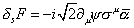
[delta]_s F = -i[square root of 2] [partial derivative]_u [psi] [sigma]^u [alpha bar]

The chiral superfields can describe spin-0 bosons, which in the Standard Model is just the Higgs boson, as well as spin-½ particles, which are the quarks and leptons of the Standard Model. However, they do not describe the spin-1 gauge bosons of the Standard Model. In order to describe spin-1 particles, the vector bosons, you need to introduce vector superfields. They are constrained to be self-conjugate.

V(X, [theta], [theta bar) = V^† (X, [theta], [theta bar])

This leads to the following representation of V.

V(X, [theta], [theta bar]) = (1 + (1/4) [theta] [theta] [theta bar] [theta bar] [partial derivative]_u [partial derivative]^u) C(x) + (i[theta] + (1/2) [theta] [theta] [sigma]^u [theta bar] [partial derivative]_u) X(x) + (i/2) [theta] [theta] [M(x) + iN(x)] + (i[theta bar] + (1/2) [theta bar] [theta bar] [sigma]^u [theta] [partial derivative]_u) [X bar] (x) – i/2 [theta bar] [theta bar] {M(x) – iN(x)] – [theta] [sigma]_u [theta bar] A^u (x) + i[theta] [theta] [theta bar] [lambda bar] (x) – i[theta bar] [theta bar] [theta] [lambda](x) + (1/2) [theta] [theta] [theta bar] [theta bar] D(x)

where C, M, N, and D are real scalars, X and λ are Weyl spinors, and A^u is a vector field. If A^u is to describe a gauge boson, V must transform as the adjoint representation of the gauge group.

Obviously, the above equation is very unwieldy, but fortunately, you now have many more gauge degrees of freedom than in non-supersymmetric theories, since now, the gauge parameters are themselves superfields. A general non-abelian supersymmetry acting on V can be described as

e^gV -> e^{-eg[capital lambda] †} e^gV e^{ig[capital lambda]}

where

[capital lambda] (x, [theta], [theta bar])

is a chiral superfield, and g is the gauge coupling.

In the case of an abelian gauge symmetry, this transformation rule can be written as

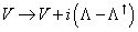
V -> V + i([capital lambda] – [capital lambda]^†)

Remember that a chiral superfield contains four scalar bosonic degrees of freedom as well as one Weyl spinor. Therefore, you can use the above transformations to choose

X(x) = C(x) = M(x) = N(x) = 0

greatly simplifying the above equation. This is called the Wess-Zumino gauge, or the W-Z gauge. It is the SUSY analog of the unitary gauge in ordinary quantum field theory since it removes any unphysical degrees of freedom. Notice that we have used only three of the four bosonic degrees of freedom in Λ. You therefore still have the ordinary gauge freedom

A_u(x) -> A_u(x) + [partial derivative]_u [psi](x)

for an abelian theory. Therefore, the W-Z gauge can be used in combination with any of the usual gauges. However, the W-Z gauge is sufficient to greatly simplify the expression for V, removing the first five terms, leaving only the last four.

If A^u has dimensions of mass, and the fermionic field has dimensions of m^3/2, that gives D the unusual dimensions of m², same as the F-component of the chiral superfield.

Applying the SUSY transformations gives a much longer expression than in the chiral superfield case so I’ll just give the following result.

[delta]_sD = -[alpha] [sigma]^u [partial derivative]_u [lambda bar] + [alpha bar] [sigma]^u [partial derivative]_u [lambda]

which shows that the D-component of a vector field transforms into a total derivative, same as the F-component of a chiral superfield.

Now let’s try to write down the supersymmetry Lagrangian. You want the action to be invariant under SUSY transformations.

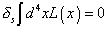
[delta]_s [integral] d⁴ x L(x) = 0

This is satisfied if L itself transforms into a total derivative. The highest components, meaning those with the largest number of θ and [θ bar] factors, of chiral and vector superfields satisfy this requirement, so you can use them to construct the Langrangian. Let’s write the action as

S = [integral] d⁴x ([integral] d² [theta] L_F + [integral] d² [theta] d² [theta bar] L_D)

where integration over Grassmann variables is defined as

[integral] d[theta]_[alpha] = 0

[integral] [theta]_[alpha] d[theta]_[alpha] = 1

with no summation over α. L_F and L_D are general chiral and vector superfields, giving rise to F-terms and D-terms respectively.

Let’s compute the product of two left-chiral superfields.

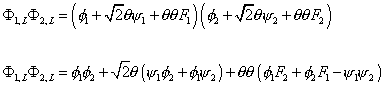
[capital phi]_{1, L} [capital phi]_{2, L} = ([phi]₁ + [square root of 2] [theta] [psi]₁ + [theta] [theta] F₁) + ([phi]₂ + [square root of 2] [theta] [psi]₂ + [theta] [theta] F₂)

[capital phi]_{1, L} [capital phi]_{2, L} = [phi]₁ [phi]₂ + [square root of 2] [theta] ([psi]₁ [phi]₂) + [theta] [theta] ([phi]₁ F₂ + [phi]₂ F₁ – [psi]₁ [psi]₂)

Since this is itself a left-chiral superfield, it does not depend on [θ bar], so it is a candidate for a contribution to the L_F term in the action. In fact, the last term looks like a fermion mass term.

If the product of two left-chiral superfields is a left-chiral superfield, the same must be true for the product of any number of left-chiral superfields. Let’s compute the highest component in the product of three such fields.

[integral] d²[theta] [capital phi]_{1, L} [capital phi]_{2, L} [capital phi]_{3, L} = [phi]₁ [phi]₂ F₃ + [phi]₁ F₂ [phi]₃ + [phi]₁ [phi]₂ F₃ – [psi]₁ [phi]₂ [psi]₃ – [phi]₁ [psi]₂ [psi]₃ – [psi]₁ [psi]₂ [phi]₃

Notice the last three terms describe Yukawa interactions between one scalar and two fermions. In the Standard Model, such interactions give rise to quark and lepton masses. Therefore, this is an interaction term in the SUSY Lagrangian. Notice that if you call φ₁ the Higgs field, ψ₂ the left-handed top quark, and ψ₃ the left-handed anti-top, the above equation will not only produce the desired Higgs-top-top interaction, but also interactions between a scalar top, called stop, the fermionic higgsino, and the top quark with equal strength. This illustrates how relations between the couplings are enforced by supersymmetry.

So far, we have identified terms that give rise to explicit fermion masses, as well as Yukawa interactions, but not yet found any terms with derivatives that can be identified with kinetic energy terms. Simply multiplying more left-chiral superfields is not going to work since that would give rise to terms with mass dimension > 4, which is nonrenormalizable. Instead, let’s consider the product of a left-chiral superfield and its conjugate, which is a right-chiral superfield. You have to be consistent in whether you’re using L-representation or R-representation. Since we’re doing this calculation in L-representation, that means you have to write the right-chiral superfield in L-representation. This gives

[[phi]_L (x, [theta])]^† = [phi]* – 2i[theta] [sigma]_u [theta bar] – 2([theta] [sigma]_u [theta bar]) ([theta] [sigma]_v [theta bar]) [partial derivative]^u [partial derivative]^v [phi]* + [square root of 2] [theta bar] [psi bar] – 2[square root of 2]i ([theta] [sigma]_u [theta bar]) [partial derivative]_u ([theta bar] [psi bar]) + [theta bar] [theta bar] F*

The product

[capital phi]_L [capital phi]_L^†

is self-conjugate, so it can be identified with a vector superfield. It is therefore a candidate for the contribution of the D-terms in the action.

[integral] d² d² [theta bar] [capital phi]_L [capital phi]_L* = FF* – [phi] [partial derivative]_u [partial derivative]^u [phi]* – i[psi bar] [sigma]_u [partial derivative]^u [psi]

This contains kinetic energy terms for the scalar component φ as well as the fermionic component ψ of chiral superfields. Notice it does not contain kinetic energy terms for F. Therefore, the F field does not propagate. It is merely an auxiliary field which can be integrated out exactly using its purely algebraic equation of motion. A chiral superfield therefore only has two physical bosonic degrees of freedom, described by the complex scalar φ. It contains equal numbers of propagating bosonic and fermionic degrees of freedom.

In order to remove the F-fields from the Lagrangian, define the superpotential f.

f([capital phi]_i) = [summation over i] k_i [phi]_i + (1/2) [summation over ij] m_ij [capital phi]_i [capital phi]_j + (1/3) [summation over i, j, k] g_ijk [capital phi]_i [capital phi]_j [capital phi]_k

where Φ_i are all left-chiral superfields, and k_i, m_ij, and g_ijk are all constants of mass dimension 2, 1, and 0 respectively. The contributions to the Lagrangian that we have mentioned so far can be written as

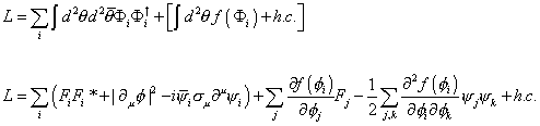
L = [summation over i] [integral] d² [theta] d² [theta bar] [capital phi]_i [capital phi]_i^† + [[integral] d² [theta] f([capital phi]_i) + h. c.]

L = [summation over i] (F_i F_i* + | [partial derivative]_u [phi] |² – i[psi bar] [sigma]_u [partial derivative]^u [psi]_i) + [summation over i] [partial derivative of f([phi]_i) with respect to [phi]_j] F_j – (1/2) [summation over j, k] [second partial derivative of f([phi]_i) with respect to [phi]_j and [phi]_k] [psi]_j [psi]_k + h. c.

where f is a function of the scalar field φ_i instead of the superfields Φ_i. Now integrate out the auxiliary fields. Their equations of motion are given by

[partial derivative of L with respect to F_j] = 0

which implies

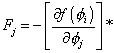
F_j = -[partial derivative of f([phi]_i) with respect to [phi]_j]*

Plugging this into the above equation for the Lagrangian gives

L = L_kinetic – [[summation over j, k] [second partial derivative of f([phi]_i) with respect to [phi]_j and [phi]_k] [psi]_j [psi]_k + h. c.] – [summation over j] | ] [partial derivative of f([phi]_i) with respect to [phi]_j] |²

The second term in the Lagrangian describes fermion masses and Yukawa interactions. The third term in the Lagrangian describes scalar mass terms and scalar interactions. Since both terms are determined by a single function f, there are many relations between the coupling constants.

The coupling of the gauge superfields to the chiral matter superfields is done by a SUSY version of the normal minimal coupling.

[integral] d² [theta] d² [theta bar] [capital phi] ^† [capital phi] -> [integral] d² d² [theta bar] [capital phi]^† e^2gV [phi] = | D_u [phi] |² – i[psi bar] [sigma]_u D^u [psi] + g[phi]* D[phi] + ig[square root of 2] ([phi]* – [lambda] [psi] – [lambda bar] [psi bar] [phi]) + | F |²

using the W-Z gauge and the normal gauge covariant derivative

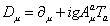
D_u = [partial derivative]_u + igA_u^a T_a

where T_a are the group generators. This part of the Lagrangian describes not only the interactions of fermions and scalars with gauge fields but also contains gauge strength interactions between fermions or higginos, ψ, Higgs bosons or sfermions, φ, and gauginos, λ. Gauginos are the supersymmetric partners of the gauge bosons.

Finally, the kinetic energy terms of the gauge fields can be described using the superfields

W_[alpha] = ([D bar]_{[alpha dot]} [D bar]_{[beta dot]} [epsilon]^{[alpha dot] [beta dot]}) e^-gV D_[alpha] e^gV

where D and [D bar] are SUSY-covariant derivatives carrying spinor superscripts. For abelian symmetries, this reduces to

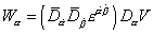
W_[alpha] = ([D bar]_{[alpha dot]} [D bar]_{[beta dot]} [epsilon]^{[alpha dot] [beta dot]}) D_[alpha] V

since

[D bar]_{[alpha dot]} [D bar]_{[alpha dot]} = 0

[D bar]_{[alpha dot]} W_[alpha] = 0

W_α is a left-chiral superfield. Its behavior under gauge transformations is the same as e^gV. The product W_α W^α is gauge invariant. It is also a left-chiral superfield, so its θ θ can appear in the Lagrangian.

(1/32g²) W_[alpha] W^[alpha] = -(1/4) F_uv^a F_a^uv + (1/2) D_a D^a + (-(i/2) [lambda]^a [sigma]_u [partial derivative]^u [lambda bar]_a + (1/2) gf^abc [lambda]_a [sigma]_u A_a^u [lambda bar]_c + h. c.)

In addition to the kinetic energy term for the gauge fields, there is also a kinetic energy term for the gauginos, as well as the canonical coupling of the gauginos to the gauge fields, determined by the group structure constants f^abc. There is no kinetic energy term for the D_a fields, so these are also auxiliary fields, and can be integrated out. Their equation of motion is

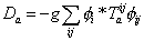
D_a = -g[summation of ij] [phi]_i* T_a^ij [phi]_ij

You also have the following contribution to the scalar interactions in the Lagrangian

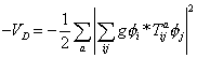
-V_D = -½ [summation over a] | [summation over ij] g[phi]_i* T_ij^a [phi]_j |²

We therefore have all the terms of the Lagrangian of supersymmetry.

If you were to go through the calculations, you would see that there are no quadratic divergences. Obviously, there are no quadratic divergences from Yukawa couplings since each chiral superfield contains equal numbers of bosonic and fermionic degrees of freedom. If you go through the calculations and determine the contributions to the Higgs self-energy due to the gauge bosons, you would see that these also cancel for the same reason. However, if you take into account hypercharge interactions, so you no longer assume that m_W = m_Z, you will find that a nonvanishing divergence remains. This is because the total trace of the hypercharge generator does not vanish. Its trace over a complete fermion or sfermion generation does vanish, but this leaves the contribution from the single Higgs doublet. The solution to this problem is to have not one but two Higgs doublets.

You need to introduce two Higgs superfields to break SU(2) x U(1). A model with a single Higgs doublet superfield has nonvanishing gauge anomalies associated with fermion triangle diagrams. The contributions from just a Standard Model fermion does vanish, but if you add a single higgsino doublet, anomalies will be introduced. You need a second higgsino doublet with opposite hypercharge to cancel the contribution from the first doublet. Also, the masses of the chiral fermions originate from terms in the superpotential. However, the superpotential can’t contain products of left and right chiral superfields. You can’t introduce a hermitian conjugate of a Higgs field, so you can’t introduce U(1) invariant terms that give mass to both type up and type down quarks, if there is only one Higgs superfield. Therefore, you need at least two doublets.

In the supersymmetry Lagrangian, the masses of the Standard Model particles are exactly the same as their supersymmetric partners. Obviously, this is not the case. We have not yet detected supersymmetric particles so their masses must be much larger than the Standard Model particles. Therefore, supersymmetry must be a broken symmetry. In the Standard Model, SU(2) x U(1) is a spontaneously broken symmetry. However, it’s not easy to break supersymmetry spontaneously. From the definition of SUSY algebra

¼ ([Q bar]₁ Q₁ + Q₁ [Q bar]₁ + [Q bar]₂ Q₂ + Q₂ [Q bar]₂) = P⁰ = H > 0

where H is the Hamiltonian. This is non-negative since it is the sum of perfect squares. If the vacuum state | 0 > is supersymmetric, then

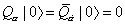
Q_[alpha] | 0 > = [Q bar]_{[alpha dot]} | 0 > = 0

so therefore

E_vac = < 0 | H | 0 > = 0

Let’s try breaking supersymmetry by the vacuum expectation value of a scalar particle, in direct analogy with SU(2) x U(1) breaking in the Standard Model. The scalar potential is given by

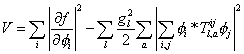
V = [summation over i] | [partial derivative of f with respect to [phi]_i] |² + [summation over l] (g_l²/2) [summation over a] | [summation over i, j] [phi]_I* T_{l, a}^ij [phi]_j |²

where l, lower case L, labels the simple groups whose product forms the entire gauge group of the model, such as SU(3) x SU(2) x U(1) in the Standard Model. You can break SUSY with either

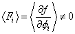
F_i = <[partial derivative of f with respect to [phi]_i] is not 0.

which is called F-breaking, or

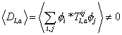
D_{l, a} = <[summation over i, j] [phi]_i* T_{l, a}^ij [phi]_j> is not 0

which is called D-breaking. The second term in the above equation for V can be minimized, meaning set to zero, if all expectation values vanish.

<[phi]_i> = 0

for all i. Turning the symmetry breaking point into the absolute minimum of the potential requires nontrivial contributions from the first term in the above equation for V.

The construction of realistic models with spontaneously broken SUSY is made even more difficult by the fact that in such models

m_{[f tilda]} = m_f

still remains satisfied on average, so at least some of the sfermions would still have masses on the order of the Standard Model particles. The supertrace over the whole mass matrix vanishes

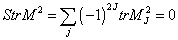
Str M² = [summation over j] (-1)^2J tr M M_J² = 0

where J is the spin, and M_J is the mass matrix for all particles of spin J. This is a problem since we want all sfermions to be significantly heavier than their Standard Model partners. You can possibly satisfy this constraint by making the gauginos very heavy, but that is also difficult to do in a self-consistent way. All potentially realistic global supersymmetry models of spontaneous SUSY breaking, where sparticles get masses at tree-level, contain a new U(1) whose D-term is nonzero in the minimum of the potential, as well as a large number of superfields beyond those required by the field content of the Standard Model. One way around this is to circumvent the above constraint by instead creating most sparticle masses only through radiative corrections, although this also requires additional superfields.

For this reason, most attempts at SUSY breaking instead do it by inserting soft breaking terms into the Lagrangian. You want to maintain the cancellation of the quadratic divergences. You have to be aware of what terms you can add to the Lagrangian that will still allow the cancellation of quadratic divergences to take place. Quadratic divergences will cancel even if you introduce the following terms.

scalar mass terms

-m_[phi]i² | [phi]_i |²

trilinear scalar interactions

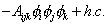
-A_ijk [phi]_i [phi]_j [phi]_k + h. c.

gaugino mass terms

-½ m_l [lambda bar]_l [lambda]_l

bilinear terms

-B_ij [phi]_i [phi]_j + h. c.

and linear terms

-C_i [phi]_i

and under certain conditions, you can add trilinear terms of the form

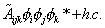
[A tilda]_ijk [phi]_i [phi]_j [phi]_k* + h. c.

where l, lower case L, labels the group factor, and h. c. is hermitian conjugate. Linear terms are gauge invariant only for gauge singlet fields. You are not allowed to introduce additional masses for chiral fermions beyond those contained in the superpotential. The relations between dimensionless coupling constants imposed by supersymmetry can’t be broken.

Let’s now look at the simplest realistic supersymmetric model. This is called the minimal supersymmetric standard model, or MSSM. It is a simple supersymmetrization of the Standard Model. You want to keep the number of superfields and interactions as small as possible. Since the Standard Model fermions are in different representations of the gauge groups than the gauge bosons, we have to place them in different superfields. No Standard Model fermion can be identified as a gaugino. One generation of the Standard Model is therefore described by five chiral superfields. Q contains quark and squark SU(2) doublets. U^c and D^c contain the quark and squark singlets. L contains the lepton and slepton doublets. E^c contains lepton and slepton singlets. The SU(2) singlet superfields contain left-handed and right-handed anti-fermions. Their scalar members have charges of +1 for [e tilda]_R^c, -2/3 for [u tilda]_R^c, and -1/3 for [d tilda]_R^c, where c denotes antiparticles. You repeat everything for each of the three generations.

Let’s look at the actual particles. In addition to the gauge bosons, you have spin ½ gaugino fields. The partners to the B_u and W_uⁱ are the [B tilda] and [W tilda]ⁱ. In the Standard Model, the W₁ and W₂ combine in one way to create W⁺, and another way to create W^–. The B_u and W₃ combine in one way to create the Z⁰ and another way to create the photon, γ. You have the same thing with the supersymmetric particles. The [W tilda] fields combine in different ways to create the positive and negative winos [W tilda]⁺ and [W tilda]^–. The [B tilda] and [W tilda] combine in one way to create the zino [Z tilda], and another way to create the photino, [gamma tilda]. The superpartners of the eight gluons are the eight gluinos, [g tilda].

Quarks and leptons have spin-0 partners called squarks and sleptons. The partner to the up quark is the up squark. The partner to the electron is the selectron. You could also identify squarks by just putting an “s-” in front of the name of the quark, so the partner to the top would be the stop, etc. Since there has to be a superpartner for each degree of freedom, two bosonic fields are needed for each Standard Model fermion. They are called the left and right states, [q tilda]_R, [q tilda]_L, [l tilda]_R, [l tilda]_L.

Lastly, you need two complex Higgs doublets with hypercharges of +1 and -1 in order to give masses to the up-type quarks, down-type quarks, and leptons, and also to cancel anomalies. The Higgs fields have spin-½ partners called higgsinos.

Superfield	Particle	Spin	Superparticle	Spin
V1	Bu	1		1/2
V2	Wui	1		1/2
V3	Gua	1		1/2
Q	(u, d)L	1/2		0
Uc		1/2		0
Dc		1/2		0
L		1/2		0
Ec		1/2		0
H1	(H10, H1–)	0		1/2
H2	(H1+, H20)	0		1/2

Now let’s write down the Lagrangian for MSSM. The gauge interactions are determined by the same gauge group as the Standard Model, SU(3) x SU(2) x U(1). Masses and couplings of the matter fields are determined by the superpotential W. The choice of gauge group constrains W but does not fix it completely. Introducing only those terms that are needed to build a consistent model, you have

W = [summation of i, j from 1 to 3] ((h_E)_ij H₁ Li E_j^c + (h_D)_ij H₁ Q_I D_j^c + (h_U) Q_i H₂ U_j^c] + uH₁ H₂

where i and j are generation indices, and we’re contracting over SU(2) and SU(3) indices.

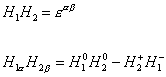
H₁ H₂ = [epsilon]^{[alpha] [beta]}

H_1[alpha] H_2[beta] = H₁⁰ H₂⁰ – H₂⁺ H₁^–

where ε^{α β} is the antisymmetric Levi-Civita tensor used to contract over the SU(2)_L weak isospin indices α, β = 1. Also

H₁ Q D^c = [epsilon]^{[alpha] [beta]} H_1[alpha] Q_[beta]^a D_a^c

where a = 1, 2, 3 are the color indices. The 3 x 3 matrices h_D, h_U, and h_E are dimensionless Yukawa couplings giving rise to quark and lepton masses. Also, h_D and h_u account for the mixing between quark current eigenstates as described by the KM-matrix. Notice the same superpotential is obtained by requiring that baryon number and lepton number be conserved, which is automatically true in the Standard Model, but not necessarily in MSSM.

You then get the following Lagrangian.

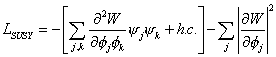
L_SUSY = -[[summation over j, k] [second partial derivative of W with respect to [phi]_j and [phi]_k] [psi]_j [psi]_k + h. c.] – [summation over j] | [partial derivative of W with respect to [phi]_j] |²

where φ_i are scalar fields, and ψ_i are fermionic fields. The first term describes masses and Yukawa interactions of fermions. The second term describes scalar terms and scalar interactions.

The interactions obtained in this way respect a symmetry called R-parity, which is defined as R = (-1)^{L + 3B + 2S}, where L is lepton number, B is baryon number, and S is spin. For normal particles, R = 1, and for their supersymmetric partners, R = -1. In confusing terminology, a particle with R = 1 is said to have even R-parity, while a particle with R = -1 is said to have odd R-parity. Normal particles, such as fermions, gauge bosons, and Higgs particles, are even, while their supersymmetric partners, which are the sfermions, gauginos, and higgsinos, are odd. Since R-parity is conserved in the MSSM, when you multiply the R-parities of the incoming particles of a Feynman diagram, it must be the same as what you get when you multiply the R-parities of the outgoing particles. Therefore, all interactions involve an even number of supersymmetric particles, or sparticles. In the supersymmetry Feynman diagrams, each trilinear vertex includes either zero or two supersymmetric partners to normal particles, which may be either incoming or outgoing particles. This means that supersymmetric particles are produced in pairs from the decay of normal particles. It also means that when a supersymmetric particle decays into two particles, one of the two is also a supersymmetric particle. Hence, in the MSSM, the lightest supersymmetric particle, or LSP, must be stable. Since LSP’s can’t decay, they must have survived from shortly after the Big Bang, before supersymmetry was broken. If the LSP was electrically charged or colored, it would bind with other particles to create exotic isotopes. Since no exotic isotopes have been detected, some people conclude that the LSP must be electrically neutral and colorless, although exotic isotopes could still exist if they were very massive. If the LSP is electrically neutral and colorless, it would be detected by the fact it carried away energy-momentum from a reaction, similar to a massive neutrino.

The LSP is an obvious candidate for dark matter. The photino, zino, higgsinos, and the axino, the supersymmetric partner of the axion, are candidates for cold dark matter. The gravitino is a candidate for warm dark matter. It should also be pointed out that conservation of R-parity is part of the MSSM, which was built on the assumption of strict minimality. However, you could come up with a more complicated SUSY model which violated conservation of R-parity, and then the LSP would not be stable after all. Which sparticle is the LSP? Many people take it to be the photino, which would be electrically neutral and colorless, although there is no way to know. It actually may be the result of a quantum mechanical mixture analogous to the KM-matrix or the neutrino mass matrix. The LSP is typically chosen to be a spin-½ particle called a neutralino, which is its own antiparticle, and is a linear combination of the photino, zino, higgsinos, and axino. In much of the parameter space, the neutralino is a bino, a particular linear combination of the photino and zino. All these possible LSP’s are weakly interacting massive particles, or WIMP’s, and would therefore be cold dark matter.

Supersymmetry allows the following vertices.

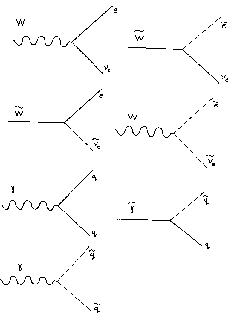
The MSSM Lagrangian, including the soft breaking terms I gave earlier, is as follows.

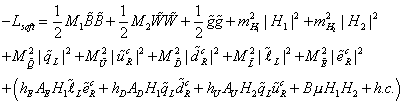
-L_soft = ½ M₁ [B tilda] [B tilda] + ½ M₂ [W tilda] [W tilda] + ½ M₃ [g tilda] [g tilda] + m_H1² | H₁ |² + m_H2 | H₂ |² + M_{[Q tilda]}² | [q tilda]_L |² + M_{[U tilda]}² | [u tilda]_R^c |² + M_{[D tilda]}² | [d tilda]_R^c |² M_{[L tilda]}² | [l tilda]_L |² + M_{[E tilda]}² | [e tilda]_R^c |² + (h_E A_E H₁ [l tilda]_L e_R^c + h_D A_D H₁ [q tilda]_L [d tilda]_R^c + h_U A_U [q tilda] [u tilda]_R^c + BuH₁ H₂ + h. c.

where M₁, M₂, and M₃ are U(1), SU(2), and SU(3) gaugino masses, m_H1², m_H2², and Bu are mass terms for the Higgs fields. The scalar mass terms M_{[Q tilda]}², M_{[U tilda]}², M_{[D tilda]}², M_{[L tilda]}² are in general hermitian 3 x 3 matrices. All the parameters are complex, so we end up with 124 free parameters, which are the masses, phases, and mixing angles. L_soft respects R-parity.

The Higgs potential gets contributions from supersymmetric F-terms, supersymmetric D-terms, and SUSY-breaking terms, which altogether give

V_Higgs = m₁² | H |² + m₂² | [H bar] |² + (m₃² H[H bar] + h. c.) + ((g₁² + g₂²)/8) (| H⁰ | – [H bar]⁰ |²) + (D-terms of H^–, [H bar]⁺)

where g₁ and g₂ are the U(1) and SU(2) gauge couplings, and the mass parameters are given by

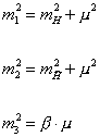
m₁² = m_H² + u²

m₂² = m_{[H bar]}² + u²

m₃² = B . u

You have

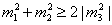
m₁² + m₂² > 2| m₃² |

so m₁² and m₃² can’t both be negative. The origin of the potential is a saddle point. In MSSM, there is a connection between gauge symmetry breaking and SUSY breaking.

You have two complex doublets H and [H bar], so you have eight degrees of freedom. Three become the longitudinal components of the W⁺, W^–, and Z⁰. That leaves five remaining degrees of freedom. They become a neutral psuedoscalar Higgs boson, two neutral scalar Higgs bosons, a positively charged Higgs boson, and a negatively charged Higgs boson. The physical psuedoscalar Higgs boson is a mixture of the imaginary parts of H⁰ and [H bar]⁰ which have the following mass matrix.

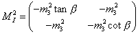
The neutral scalar Higgs bosons are mixtures of the real parts of H⁰ and [H bar]⁰ which have the following mass matrix

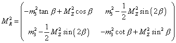
Also, the ratio of the vacuum expectation values of the Higgs fields is given by

tan[beta] = [v bar]/v

The MSSM allows for gauge coupling unification at M_X = 10¹⁶ GeV, consistent with grand unified theories. The gauginos are in the same representation of the gauge group. The gaugino masses are also unified at scales Q > M_X. The one loop renormalization group equations for the gauge couplings and gaugino masses are

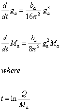
d/dt g_a = (b_a/16[pi]²) g_a³

d/dt M_a = (b_a/8[pi]²) g_a² M_a

where

t = ln (Q/M_a)

and the b_a coefficients are given by

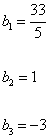
b₁ = 33/5

b₂ = 1

b₃ = -3

For comparison, the b_a coefficients for the Standard Model are

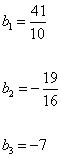
b₁ = 41/10

b₂ = -19/16

b₃ -7

The difference is due to the fact that the MSSM has a richer particle spectrum in the loops. Therefore, for the MSSM, you have

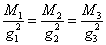
M₁/g₁² = M₂/g₂² = M₃/g₃²

at any renormalization group scale up to two loops.

The supersymmetry breaking scale should be around 1 TeV, so supersymmetric particles should be around that mass, in which such case they will be detectable by the Large Hadronic Collider at CERN.

Supersymmetry can also be used as the basis of another mechanism to provide the baryon asymmetry of the Universe, called the Affleck-Dine mechanism. Let’s say you have a colorless electrically neutral combination of quarks and leptons. This object then has a supersymmetric scalar partner, X, that is a combination of squark and slepton fields. In supersymmetric field theories, you have flat directions in field space where the scalar potential vanishes. There are directions in the superpotential along which X is a free massless field. During inflation, the X field is displaced, causing initial conditions for the evolution of the field. There are baryon number violating operators in the potential V(X) which determine the initial phase of the field. You then end up with baryon number violation which could explain the baryon asymmetry of the Universe.

Up to this point, we’ve only considered the simplest type of supersymmetry, called N = 1 supersymmetry. N measures the number of supersymmetric generators. If you have the supersymmetry generator Q that we’ve been discussing so far, that’s called N = 1 supersymmetry. If you double the number of supersymmetry generators, that’s N = 2 supersymmetry. If you double it again, that’s N = 4 supersymmetry. If you double it again, that’s N = 8 supersymmetry. N = 8 is the highest N considered, since higher N would produce particles with spin more than two, and the graviton, which is spin-2, is considered the highest spin particle in existence. Thus, N can take values of 1, 2, 4, or 8. The number of particles in a supermultiplet is 2^N. For N = 1, that gives 2¹ = 2 particles, one of which is a normal particle, and the other of which is its supersymmetric partner. For N = 2, that gives 2² = 4 particles, one of which is a normal particle, and the other three of which are its supersymmetric partners. In N = 1 supersymmetry, a spin-1 particle has one supersymmetric partner which is spin-½. In N = 2 supersymmetry, a spin-1 particle has three supersymmetric partners, two of which are spin-½, and one of which is spin-0. As you can see, the number of supersymmetric particles rises very rapidly as N increases. However, there are some advantages to considering N > 1. For instance, in N = 4, the beta function is zero.

So far I have discussed grand unified theories and supersymmetry. It’s natural to combine these two basic extensions of the Standard Model together. They work better in conjunction than either does alone. There are two basic ways of doing this. One is to take a supersymmetric theory, and embed it within a grand unified theory. The second is to take a grand unified theory, and come up with a supersymmetric version of that. If you supersymmetrize the Standard Model, you get the minimal supersymmetric standard model, or MSSM. If you supersymmetrize SU(5) grand unified theory, you get supersymmetric SU(5). For instance, the X and Y bosons now have supersymmetric partners called xinos and yinos. You have chiral and vector superfields belonging to the [5 bar]-dimensional and 10-dimensional representations. You need the two sets of Higgs superfields belonging to the 5-dimensional and [5 bar]-dimensional representations of SU(5) to generate the fermion masses. You also need the 24-dimensional Higgs field to break the SU(5) group down to SU(3) x SU(2) x U(1). All other fields are supersymmetric generalizations of the fields present in SU(5). The rate of X and Y exchange is determined by their masses, which are determined by the unification scale, which changes when you add supersymmetry, since the renormalization group is different, due to the contributions of both fermions and bosons to the self-energy. Now, in supersymmetry, F-terms can give rise to baryon number violation. Still, the proton lifetime is longer in supersymmetric SU(5) than in normal nonsupersymmetric SU(5). That’s an additional advantage of supersymmetry. You can also come up with supersymmetric SO(10). It should be emphasized that both SU(5) and SO(10) suffer from the hierarchy problem, which can only be solved by supersymmetry.

Up until now, we have assumed that supersymmetry was a global symmetry. However, like everything else in physics, it should be a local symmetry. Distant parts of the Universe that aren’t casually connected shouldn’t be forced to have the same values for various quantities. Remember in my paper on the Standard Model where I talked about making the Lagrangians locally invariant? You have to add extra terms to cancel out the unwanted derivative terms that destroy local invariance, and those added terms can be identified with the gauge bosons. The same thing happens when you try to make supersymmetry locally invariant. If ε is a spinor that generates the SUSY transformations, the gauge invariance will be spoiled by terms involving

[partial derivative]^u [epsilon]

Therefore, you have to add a new gauge field X^u to cancel out the derivative term

[delta]X is proportional to [partial derivative]^u [epsilon]

This gauge boson has a spin of 3/2. You can imagine that this new particle is a supersymmetric partner of another particle with spin-2. You can call this spin-2 particle the graviton, and the spin-3/2 particle, the gravitino. This is an amazing result. Just by making supersymmetry locally invariant, you arrive at a theory that naturally includes gravity. This theory is called supergravity. Supergravity with N > 1 is called extended supergravity. Unfortunately, supergravity is non-renormalizable. All pre-string attempts to quantize gravity are non-renormalizable, and supergravity does nothing to address this problem.

The idea that transformations should be invariant under local coordinate change is of course one of the main principles of general relativity, so in a odd way, you are including an aspect of general relativity in supersymmetry by making it locally invariant, and then as a result, it predicts a spin-2 particle we can identify with the graviton. Unfortunately, any spin-2 point particle gives a non-renormalizable theory, whether it arises naturally, or you put it in by hand. However, there are advantages to supergravity beyond the fact that it predicts the graviton. The difficulties in coming up with spontaneous symmetry breaking for supersymmetry are derived from the fact that supersymmetry is a global symmetry. However, in supergravity, supersymmetry is a local symmetry, so you don’t have that problem.

The following is the Kahler potential.

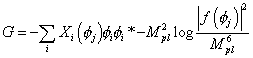
G = -[summation over i] X_i ([phi]_j) [phi]_i [phi]_i* – M_pl² log (|f([phi]_j)|²/M_pl⁶

where f is the superpotential, and X_i are real functions of the chiral fields φ_j. Supersymmetry is broken spontaneously if

G_i = [partial derivative of G with respect to [phi]_i] is not equal to 0.

It is difficult to break supersymmetry using only the fields in the MSSM. Therefore, you introduce a hidden sector which consists of some fields that do not have any gauge or superpotential couplings to the visible sector of the MSSM. The number of free parameters can be greatly reduced by imposing a global U(N) symmetry on the Kahler metric, where N is the number of superfields in the visible sector. Since the MSSM has so many free parameters, this is an additional benefit of supergravity.

Supergravity naturally predicts a spin-2 particle that can be identified with the graviton, but doesn’t change the fact that any theory that contains a spin-2 particle is non-renormalizable. In fact, throughout most of the 20th Century, any attempt to quantize gravity was non-renormalizable. This was a problem endemic in all attempts to quantize gravity. Obviously, this problem required a very radical innovative solution. This solution turned out to be string theory. Up until this point, we have assumed that particles were zero-dimensional points. String theory rests instead on the premise that particles are one-dimensional line segments. If the end points of a line segment meet, they can join to form a little loop. Line segments are called open strings, and loops are called closed strings. The way a string oscillates determines what type of particle it appears as. Point particles sweep out world lines, and their Feynman diagrams are networks of lines that meet at vertices. Strings sweep out two-dimensional world sheets or tubes. Their Feynman diagrams are surfaces or tubes that join smoothly without corners.

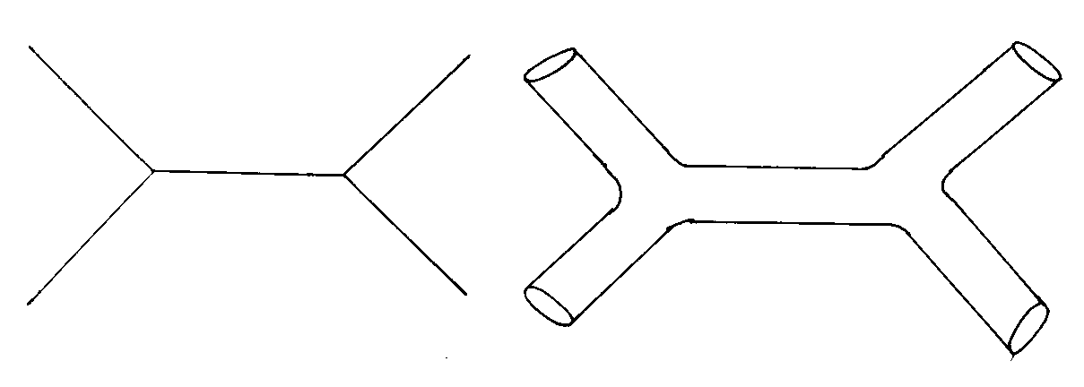
The non-renormalizable infinities originate from trying to describe a spin-2 particle at the vertex of a Feynman diagram. Since there are no vertices in the Feynman diagrams of strings, you don’t have that problem. Therefore, you can have a quantum theory of gravity, and successfully unite gravity with the other forces. Not only that, but string theory actually predicts a massless spin-2 particle. String theory plus supersymmetry is called superstring theory. Superstring theory has achieved the ultimate Holy Grail of 20th Century physics, which is one renormalizable quantum theory that accurately describes all four forces of nature, including gravity.

For this reason, superstring theory has been called a “theory of everything”. However, some string theorists disagree with that phrase. First of all, it’s still a work in progress. We have not yet arrived at a final fully predictive version of superstring theory. Second of all, even when we have a final comprehensive predictive superstring theory, it will not be the final word in physics. It will contain free parameters or so-called fundamental constants that will need further explanation as to why they have the values they do. For instance, what determines which specific manifold the extra dimensions are compactified on? If you look throughout the history of physics, from Ancient Greece to the present day, everyone always assumes that their view of the Universe is close to the truth, and they were close to the final theory of physics. Obviously, that kind of wishful thinking has never been true in the past, it’s not true now, and it will never be true in the future. Third of all, superstring theory is useful in many fields of advanced physics, from cosmology to black holes, but no one should expect it to answer every question in every field of physics, and there are some fields, such as chaos theory, that should not benefit from superstring theory at all. Therefore, superstring theory is not a literally a “theory of everything”. Having got that disclaimer out of the way, if I may regain the spirit of the previous paragraph, superstring theory ranks among the greatest intellectual achievements of mankind. Nothing should detract from the enormous success that superstring theory has achieved. That success is even more astounding considering the humble origins and history of string theory.

In the 1950’s, electromagnetism was very accurately described by QED, but there was no analogous theory for the strong force which acted between the multitude of hadrons, which were at that time considered fundamental. One attempt to describe the strong force was the S-matrix approach, which was originally founded in quantum field theory, but had since evolved into the boot-strap formulation, which was an anti-field theory approach. One strand of S-matrix development was Regge theory, which came to dominate the analysis of the high energy regime. However, then came along the quark model of Murry Gell-Mann and George Zweig, which led to QCD, which was an extremely successful theory of the strong force. Previous alternative theories of the strong force, such as Regge theory, fell by the wayside as defunct historical curiosities.

In 1968, Gabriele Veneziano published a paper on the dual resonance model derived from Regge theory. In the period 1968 – 1973, there were just a few people working on this obscure offshoot of Regge theory. After a couple of years of working on it, it slowly dawned on them that their theory assumed that hadrons were one-dimensional line segments instead of zero-dimensional points, which at the time must have seemed bizarre. In 1970, Yoichiro Nambu, Leonard Susskind, and Holger Nielson determined that this dual resonance model actually requires that particles be thought of as strings. Lenny Susskind claims that for one day, he was the only person in the world who knew it was a theory of strings. At any rate, no one could get the damn thing to work. For one thing, it assumed there were extra spatial dimensions, which they considered obviously impossible. Second of all, the theory was plagued with a massless spin-2 particle, which they considered an aberrant defect, and they couldn’t figure out how to get rid of it. Then came along QCD, which was a beautiful successful description of the strong force, so this obscure offshoot of the now defunct Regge theory was dropped by its few adherents.

It was genius of John Schwarz and Joel Scherk of Cal Tech, in 1974, and independently of Tamiaki Yoneya, to recognize the hidden potential of this ugly duckling theory. If this theory naturally has a massless spin-2 particle in its spectrum, which obviously can be identified with the graviton, that raises the hope of possibly being able to unite gravity with the other forces. Instead of hadrons, which were no longer considered fundamental, they imagined that the Standard Model particles were actually strings. If the theory includes gravity, then the string length would be close to the Planck length, which would explain why we detect them as point particles. Also, the extra dimensions would be compactified on the same very small distance scales, which would explain why we don’t detect them either. The tension of a string is analogous to the mass of a point particle.

Still, there were serious drawbacks to the first string theory. It only describes bosons, with no fermions at all. It assumed 26 spacetime dimensions. Also, it predicted the existence of a tachyon, assumed to be impossible. However, these problems are solved if you combine string theory with supersymmetry. Supersymmetry would create fermionic partners to the bosons, thus allowing fermions. In superstring theory, there were 10 spacetime dimensions instead of 26. Also, supersymmetry removed the tachyon from the spectrum. Despite this, few people studied superstrings from 1974 – 1984.

During the first superstring revolution, from 1984 – 1985, string theory was transformed from an obscure theory to the forefront of theoretical particle physics. During this time, it was realized that there are actually five different superstring theories, described as follows.

Type	Open versus Closed	Gauge Group	Parity	Supersymmetry	S dual	T dual
Type I	open and closed	SO(32)	violating	one supersymmetry	Heterotic SO(32)	Type IA
Type IIA	closed	U(1)	conserving	two supersymmetries	none	Type IIB
Type IIB	closed	none	violating	two supersymmetries	Type IIB	Type IIA
Heterotic SO(32)	closed	SO(32)	violating	right-movers supersymmetric left-movers not	Type I	Heterotic E8 x E8
Heterotic E8 x E8	closed	E8 x E8	violating	right-movers supersymmetric left-movers not	none	Heterotic SO(32)

Type I strings are open, and the rest are closed. Of course, if the ends of an open string meet, it forms a closed string, so Type I includes both open and closed strings, while the others include only closed strings. For closed strings, the oscillations of the string, which are little waves on the string itself, can move either to the left or to the right. Waves that move counterclockwise around the loop are called left-movers, and waves that move clockwise around the loop are called right-movers. Left-movers and right-movers do not interfere with each other. For Type IIA and Type IIB superstrings, both the left-movers and right-movers are supersymmetric. For the two heterotic superstring theories, the right-movers are supersymmetric, and the left-movers are non-supersymmetric. Type IIA is parity conserving, in contradiction to reality, although later it was figured out how to induce parity violation in the compactification process. The heterotic strings were discovered in 1984 by Gross, Harvey, Martinec, and Rohm.

The second superstring revolution, from 1994 – present, brought non-perturbative string physics within reach. It was realized that the five string theories are related to each other through dualities. If theory A at strong coupling, meaning with a large strength of interaction, is equivalent to theory B at weak coupling, they are S-dual. If theory A compactified on a space of large volume is equivalent to theory B compactified on a space of small volume, they are T-dual. If theory A compactified on a space of large volume is equivalent to theory B at strong coupling, they are U-dual. T-duality, unlike S-duality or U-duality, can be understood perturbatively, and thus was discovered between the two string revolutions. If two theories A and B are S-dual, they are related by

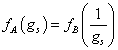
f_A (g_s) = f_B = (1/g_s)

where g_s is the string coupling constant. Two of the superstring theories, Type I and Heterotic SO(32), are related by S-duality. Type IIB is self-dual under S-duality. Thus, S-duality is a symmetry of Type IIB theory. This symmetry is broken if g_s = 1. Because of S-duality, the strong coupling behavior of each of these three theories is determined by a weak coupling analysis. The remaining two theories, Type IIA and Heterotic E₈ x E₈ behave very differently at strong coupling. They change from 10-dimensional to 11-dimensional.

If two theories are T-dual, they are related by

R_A R_B = (l_s)²

where R is the radius of the compactified dimension, and l_s is the string length. When one of the circles becomes small, the other becomes large. Type IIA and IIB are T-dual to each other. Heterotic SO(32) and Heterotic E₈ x E₈ are T-dual to each other. These various dualities led to the conclusion that all five string theories are related to each other, and are in fact, just limiting cases of a single underlying theory, that we now usually call M-theory.

Until 1995, it was only understood how to formulate string theories in terms of perturbation expansions. Perturbation theory is useful in a quantum theory that has a small dimensionless coupling constant, since it allows you to compute physical quantities as power series expansions in the small parameters. For a physical quantity T(α), you compute using Feynman diagrams.

T([alpha]) = T₀ + [alpha] T₁ + [alpha]² T₂ + …

For QED, the fine structure constant is

[alpha] ~ 1/137

For QED, this process works because α is so small. Each term is much smaller than the previous term, so you can neglect higher terms. However, more generally, there are various non-perturbative contributions, such as instantons, that have the structure

T_NP ~ e^-(c/[alpha])

where c is a constant. In QCD, at high energy, perturbation theory is useful due to asymptotic freedom. At low energy, it is not, due to confinement, and you have to use other methods, such as lattice QCD.

In string theory, the dimensionless string coupling constant, g_s, is determined dynmamically by the vacuum expectation value of a scalar field called the dilaton. Right now, it’s essentially a free parameter you can make anything you want, but there is no reason to assume that it is small. Therefore, it’s good to be able to study string theory non-perturbatively.

The other major advance of the second superstring revolution was the study of the boundary conditions of open strings. There are 10 dimensions, 9 of space, and one of time. Let’s say the end points of an open string can propagate freely through all spatial dimensions. These are called Neumann boundary conditions. However, the endpoints of an open string could also be fixed, and not free to move. This is called Dirichlet boundary conditions. The endpoint of an open string could be fixed in some dimensions and not others. For instance, it could be fixed in seven of the nine spatial dimensions, and free to move in the other two. It would then be free to slide around in a two-dimensional plane. That two-dimensional surface could then be considered a physical object called a Dirichlet membrane, or D-brane. If the endpoints of an open string had p Neumann boundary conditions, it therefore has 9 – p Dirichlet boundary conditions, and ends on a Dp-brane.

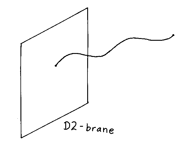
You could think of a string as simply a 1-brane, although remember that branes are defined in terms of strings ending on them, whereas strings are postulated from the beginning. D-branes were discovered/invented by Joseph Polchinski in 1995.

All the string theories have a second rank tensor field called B_uv, called the Kalb-Ramond field. A particle, such as an electron, can be charged under the photon field, which is a vector field A_u, which then gives the electron stability, due to conservation of charge. In the same way, strings themselves are charged under the second rank tensor field B_uv, and this gives strings stability.

Since string theory talks a lot about compactifying spaces, I should discuss some basic topology. I said at the beginning of my paper on the Standard Model, that mathematicians try to go from the specific to the general. In geometry, that takes the form of topology. In traditional geometry, a regular polygon is considered the same shape if you do a translation, rotation, or reflection, but not if you do a deformation, such as changing the angles, the lengths of the sides, the number of sides, or the curvature of the sides, from flat to curved. Topology uses an expanded definition of “same shape”, so it is still considered the same shape under the other manipulations I listed. All regular polygons, irregular polygons, a circle, an ellipse, etc. are all considered the same shape, which for simplicity, is represented by the circle. In other words, they are topologically equivalent.

Special relativity assumes a flat background metric called Minkowski space. General relativity generalizes this by allowing curved space. This potentially curved space is called a manifold. The simplest manifold is flat space. In geometry, this is called Euclidean space, or Rⁿ, the set of n-tuples (x₁, x₂, …x_n) More generally, a manifold is a space that locally looks like Rⁿ. The space may be curved and have a complicated topology, but in local regions, it looks just like Rⁿ. The entire manifold is constructed by smoothly sewing together these local regions. The simplest manifold is, of course, n-dimensional Euclidean space, Rⁿ, since it obviously looks like Rⁿ not just locally but globally. A one-dimensional line is called R¹. A two-dimensional plane is R². Three-dimensional space is R³.

The second simplest manifold is the n-sphere, Sⁿ. This is defined as the locus of all points some fixed distance from a given point in R^{n + 1} space. A circle is called S¹. A sphere, which topologists call a two-sphere, is S². A hypersphere, or three-sphere, is S³. Notice n is the dimensionality of the surface, not the entire thing which exists in n + 1 dimensions.

The next simplest manifold is the n-torus, Tⁿ. A torus is a surface of revolution formed by a circle being rotated about a coplanar line outside the circle. You can form a torus from a square or rectangle. Imagine, you have a square, and you roll it up and join two opposite sides, and form a cylinder. Then you bend the cylinder into a circle, and attach the two opposite ends to form a torus. More generally, an n-torus, Tⁿ is formed by taking an n-dimensional cube, and attaching all opposite sides to each other. What we normally think of as a torus is called a two-torus or T².

A torus has one hole. However, an acceptable manifold could have any number of holes. You can represent the number of holes in a torus by the genus. A Riemann surface of genus g is a two-torus with g holes instead of one. A sphere, S², is a Riemann surface of genus zero. A two-torus, T², is a Riemann surface of genus one. A torus-like shape with two holes is a Riemann surface of genus two. Every compact orientable boundaryless two-dimensional manifold is a Riemann surface of some genus.

The genus 2 manifold is called a double-torus, or the connected sum of two tori, and is symbolized by T² # T². All of the above manifolds are orientable manifolds, which means they have two sides. If you look at a plane, R², you’re either on one side or the other. If you have a sphere, S², any point not on the surface is either inside or outside. An example of a non-orientable manifold would be a klein bottle, K² or KB, which only has one side to it. It was invented by Felix Klein in 1882. Despite what it may look like in the diagram, it does not intersect itself. It uses the fourth spatial dimension to jump over itself.

If a manifold extends infinitely, such as a line or plane, it is called non-compact. If a manifold has a finite area, such as a circle, sphere, or torus, it is called compact. A manifold does not have to be a geometric shape. A set of continuous transformations, such as rotations in Rⁿ, forms a manifold. Lie groups are manifolds with group structure. Also, the direct product of two manifolds is a manifold. If you take two manifolds M and M’ of dimensions n and n’, you can construct a manifold M x M’ of dimension n + n’.

A manifold could have no boundaries, such as a line, circle, plane, sphere, or all the other examples I’ve listed so far, or it could have boundaries, such as an interval, disk, ball, finite cylinder, Möbius strip, or “pair of pants”.

What is not a manifold? A topology is not a manifold if there is somewhere that is does not locally look like Rⁿ. Examples include a one-dimensional line attached to a two-dimensional plane, or two cones attached at the vertices.

Now let’s look at an example of a product of two manifolds. Let’s say one is a line, R¹, and the other is a circle, S¹. Since each is one dimensional, their product would be 1 + 1 = 2 dimensional. Their product would be R¹ x S¹, which is an infinite cylinder. Notice that the cross section along the axis of the cylinder is parallel lines, each of which is R¹, and the cross section perpendicular to the axis of the cylinder is a circle, which is S¹.

If the radius of the circle was very small, the cylinder would be indistinguishable from a line. Imagine a rubber garden hose. On a scale of tens of meters, it can be treated as a one-dimensional line. On a scale of centimeters, it looks like a two-dimensional surface, although you can still detect the curvature, and it should be treated like a cylinder. On a scale of a millimeter or less, you could treat it like a flat plane. You see how on a scale of tens of meters, it appears one-dimensional when it’s really a two-dimensional surface. Thus, if one of the dimensions is compactified on a circle the radius of which is very small compared to the size scale at which you’re looking at, it would appear to have one less dimension. R¹ x S¹ would look like R¹ if the radius of S¹ was very small. If you were in a R³ x S¹ manifold, which is four-dimensional, and the radius of S¹ was the Planck length, you would think you were in a R³ manifold, which is three-dimensional. In this way, the 10-dimensional spacetime assumed in string theory appears to us as 4-dimensional spacetime. The other six dimensions are compactified on a scale of the Planck length,10^-35 meters, so obviously we can’t detect them.

Since the equations must be satisfied, the geometry of the six-dimensional space is not arbitrary. What works best is a type of manifold called a Calabi-Yau manifold, which is a Kahler manifold with vanishing first Chern class. In 1954, Eugenio Calabi first theorized the possibility of such a thing. In 1976, Shing-Tung Yau proved the Calabi conjecture, and discovered Calabi-Yau space. In 1985, Candelas, Strominger, Horowitz, and Witten proposed that the extra dimensions required by string theory could be compactified on a Calabi-Yau manifold. You can’t draw a picture of it since it’s six-dimensional, and has no analog is three dimensions. Calabi-Yau compactification, in the context of E₈ x E₈ heterotic superstring theory, can give a low energy effective theory that closely resembles a supersymmetric extension of the Standard Model. Superstring theory, therefore usually assumes that our Universe corresponds to a M x CY manifold, where M is Minkowski space, and CY is a Calabi-Yau manifold. There are several Calabi-Yau spaces, and if you choose the one with the correct topology, the resulting theory predicts that you should have three generations of quarks and leptons. It is very encouraging that you can get the right results by choosing the correct topology, although you would prefer to have a deeper motivation for why you choose that topology. In other words, you can choose the values of free parameters to fit what you observe, although the question remains as to why they have those values.

A Joyce manifold, or Riemannian manifold with G₂ holonomy, is a 7-dimensional manifold for which each tangent space is equipped with all the structure of the imaginary octonions. M-theory is an 11-dimensional theory, and you can compactify seven of the dimensions on a Joyce manifold in order to leave the four spacetime dimensions we’re familiar with.

It is worthy of mention that the idea of uniting gravity with the other forces by assuming extra compactified dimensions goes back to the work of Theodore Kaluza in 1919, and later expanded by Oskar Klein in 1926. At that time, the only other force known was electromagnetism. In Kaluza-Klein theory, the extra dimension in a five-dimensional version of general relativity is compactified on a circle, giving rise to a new local U(1) symmetry which can be identified with electromagnetism. Of course, it was actually easier to unite gravity and electromagnetism at that time, since they didn’t have to develop a quantum theory of gravity, since quantum theory itself had not yet been invented. Indeed, it was the invention of quantum mechanics, and the inability to quantize gravity, which was why Kaluza-Klein theory didn’t really go anywhere, although the view of modern physics has some similarities to some aspects of it.

Any theory that unites gravity with quantum field theory must involve the three fundamental constants, the universal gravitational constant, G = 6.674215 x 10^-11 Nm²/kg² or m³/kgs², Planck’s constant, h = 6.626176 x 10^-34 Js, or [h bar] = h/2π = 1.05 x 10^-34 Js, and the speed of light, c = 2.99792458 x 10⁸ m/s. These three fundamental constants can be combined to create quantities with the units of mass, length, and time. They are called the planck mass, planck length, and planck time.

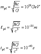
m_pl = [square root of ([h bar]c/G)] = 10¹⁹ GeV

l_pl = [square root of ([h bar]G/c³)] = 10^-35 m

t_pl = [square root of ([h bar]G/c⁵)] = 10^-43 s

Max Planck first listed his set of units in May 1899 in a paper presented to the Prussian Academy of Sciences. The planck time is the smallest unit of time it’s possible to talk about. The planck length is the smallest unit of length it’s possible to talk about. The planck mass is the highest energy scale it’s possible to talk about. The planck time after the Big Bang, the Universe had a energy of the planck mass, and at that energy, gravity had the same strength as the other forces, which is the same as the situation today at distances as short as the planck length. The extra dimensions would be compactified on the scale of the planck length. The string length might also be at that scale, or might be two orders of magnitude larger, which is still so small that they would appear as point particles to us.

Remember that E = mc² so in naturalized units where c = 1, E = m, which is why we can measure mass in units of energy, such as electron volts. In this context, the planck mass, 10¹⁹ GeV, is of fundamental significance as the highest possible energy scale, and the scale at which gravity is as strong as the other forces. If instead, you measure the planck mass in units of mass, you get 10^-8 kilograms, which is about the mass of biological cell, and has no cosmological significance. People have also come up with various derived planck units. The planck temperature T_pl = (c⁵[h bar]/G)^1/2/k = 10³² Kelvin, is the temperature of the Universe a planck time after the Big Bang, where k is Boltzmann’s constant. The planck density is ρ_pl = m_pl/(l_pl)³ = 10⁹⁶ kg/m³ is the density of the Universe a planck time after the Big Bang. The planck force is F_pl = c⁴/G = 10⁴³ newtons, and some have suggested that this could be the tension of a string. The planck area is the square of the planck length, and the planck volume is the cube of the planck length.

Before we look at strings in more detail, let’s review the familiar case of a traditional point particle. In what follows, we’ll use the variable

x_u ([sigma], [tau])

where σ parametrizes the position of a point on a string, and τ gives the time evolution. Since a point particle doesn’t have a position on a string, you just have

x^u ([tau])

that describes how the world line, parametrized by τ, is embedded in the spacetime, whose coordinates are given by x^u. For simplicity, let’s assume that spacetime is flat Minkowski space with a Lorentz metric.

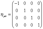
n_uv = Diag [-1, 1, 1, 1]

You could, of course, assume a curved spacetime by replacing n_uv by a metric g_uv (x). Assuming Minkowski space, the Lorentz invariant world line element in given by

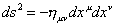
ds² = -n_uv dx^u dx^v

Assuming [h bar] = c = 1, the action for a particle of mass m is given by

S = -m [integral] ds

In terms of the embedding functions x^u (t), the action can be rewritten in the form

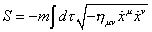
S = -m [integral] d[tau] [square root of (-n_uv [x dot]^u [x dot]^v)]

where dots represent τ derivatives. This action is invariant under local reparametrizations. This is a kind of gauge invariance, where the form of S is unchanged by an arbitrary reparametrization of the world line.

[tau] -> [tau] ([tau tilda])

We require that the function τ ([τ tilda]) is smooth and monotonic.

[derivative of [tau] with respect to [tau tilda]] > 0

The reparametrization invariance is a one-dimensional analog of the four-dimensional general coordinate invariance of general relativity. This kind of symmetry is called diffeomorphism invariance.

The reparametrization invariance of S allows you to choose a gauge. Let’s choose the static gauge.

x⁰ = [tau]

In this gauge, renaming the parameter t, the action becomes

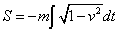
S = -m [integral] [square root of (1 – v²)] dt

where

v = [derivative of x with respect to t]

Requiring this action to be stationary under an arbitrary variation of x (t) gives the Euler-Lagrange equations.

[derivative of p with respect to t] = 0

where

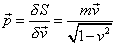
p = [delta]S/[delta]v = (mv)/([square root of (1 – v²)]

The usual relativistic kinematics follows from the action

S = -m [integral] ds

Now, let’s take what we just did for a point particle, and do the same thing for a p-brane of tension T_p. For p = 0, you have a 0-brane, which is a point particle. For p = 1, you have a 1-brane, which is a string. You could think of it as a generalization of what we just did, except we are no longer assuming p = 0. For p = 0, the tension T_p is what we call the mass. Just as a point particle sweeps out a world line, a p-brane sweeps out a world-volume with p + 1 dimensions. The action in this case involves the invariant (p + 1)-dimensional volume, and is given by

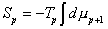
S_p = -T_p [integral] du_{p + 1}

where the invariant volume element is

du_{p + 1} = [square root of (- det (-n_uv [partial derivative]_[alpha] x^u [partial derivative]_[beta] x^v) d^{p + 1} [sigma])]

Here the embedding of the p-brane into d-dimensional spacetime is given by the functions x^u (σ^α). The index α = 0, 1, …p labels the p + 1 coordinates σ^α of the p-brane world volume, and the index u = 0, 1, …d – 1 labels the d coordinates x^u of the d-dimensional spacetime. You have

[partial derivative]_[alpha] [partial derivative of x^u with respect to [sigma]^[alpha]]

The determinant acts on the (p + 1) x (p + 1) matrix whose rows and columns are labeled α and β. The tension T_p is the mass per unit volume of the p-brane. For a 0-brane, meaning a point particle, it’s just the mass.

S[x] = -T [integral] d[sigma] d[tau] [square root of ([x dot]² x’² – ([x dot] . x’)²]

where

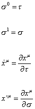
[sigma]⁰ = [tau]

[sigma]¹ = [sigma]

[x dot]^u = [partial derivative of x^u with respect to [tau]]

x’^u = [partial derivative of x^u with respect to [sigma]]

This action is called the Nambu-Goto action, and was first proposed by Yoichiro Nambu and Goto in 1970.

The Nambu-Goto action is equivalent to the Polyakov action

S[x, h] = -(T/2) [integral] d² [sigma] [square root of -h] h^{[alpha][beta]} n_uv [partial derivative]_[alpha] x^u [partial derivative]_[beta] x^v

where

h_{[alpha] [beta]} ([sigma], [tau])

is the world-sheet metric, and h = det h_{α β}. The Euler-Lagrange equation obtained by varying h^{α β} is

T_{[alpha] [beta]} = [partial derivative]_[alpha] x . [partial derivative]_[beta] – (1/2) h_{[alpha] [beta]} h^{[gamma] [delta]} [partial derivative]_[gamma] x . [partial derivative]_[delta] x = 0

In addition to reparametrization invariance, the action S[x, h] has another local symmetry called conformal invariance or Weyl invariance. It is invariant under the following transformation

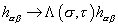
h_{[alpha] [beta]} -> [capital lambda] ([sigma], [tau]) h_{[alpha] [beta]}

This local symmetry is unique to strings, meaning the p = 1 case. These two reparametrization invariance symmetries of S[x, h] allow you to choose a gauge in which the three functions h_{α β}, which is a symmetric 2 x 2 matrix, are expressed in terms of just one function. You can write the conformally flat gauge

h_{[alpha][beta]} = n_{[alpha][beta]} e^{[phi]([sigma], [tau])}

where η_{α β} is the two-dimensional Minkowski metric on a flat world sheet. However, because of the factor e^φ, h_{α β} is only conformally flat. Using this gauge choice for S[x, h] leaves the gauge-fixed action

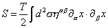
S = (T/2) [integral] d² [sigma] n^{[alpha] [beta]} [partial]_[alpha] x . [partial derivative]_[beta] x

However, this does not take into account quantum mechanics. You should perform a Feynman path integral. When you do this, you find that φ does not decouple from the answer. It only works when d = 26. Otherwise, there are correction terms that can be traced to a conformal anomaly, meaning a quantum mechanical breakdown of the conformal invariance.

The gauge-fixed equation is quadratic in the x’s. It is the same as a theory of d free scalar fields in two dimensions. The equations of motion obtained by varying x^u are simply free two-dimensional wave equations.

[x double dot]^u – x”^u = 0

You also have to take into account the constraints, T_{α β} = 0, which are

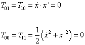
T₀₁ = T₁₀ = [x dot] . x’ = 0

T₀₀ = T₁₁ = ½ ([x dot]² + x’²) = 0

which gives you

([x dot] ± x’)² = 0

We saw that d = 26, meaning the bosonic string theory has 26 dimensions. Let’s show in more detail why this is. If α₀ is the vacuum energy, you evaluate it using the following regularization.

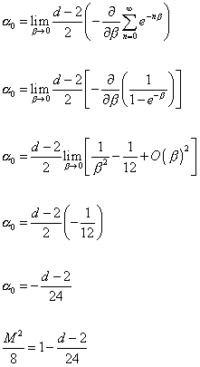
[alpha]₀ = lim [beta] -> 0 ((d-2)/2) (-[derivative with respect to [beta]] [summation over n to infinity] e^-n[beta])

[alpha]₀ = lim [beta] -> 0 ((d-2)/2) (-[derivative with respect to [beta]] (1/(1 – e^-[beta])))

[alpha]₀ = ((d – 2)/2) lim [beta] -> 0 [(1/[beta]²) – (1/12) + O([beta])²]

[alpha]₀ = ((d – 2)/2) (-1/12)

[alpha]₀ = -(d – 2)/24

M²/8 = 1 – (d – 2)/24

The only way this level is compatible with Lorentz invariance is if this level is massless. In the above equation M = 0 only if d = 26. Therefore, the bosonic string requires 26 spacetime dimensions.

Next, we will discuss the boundary conditions. A string can be open or closed. If it’s open, it could have either Neumann or Dirichlet boundary conditions.

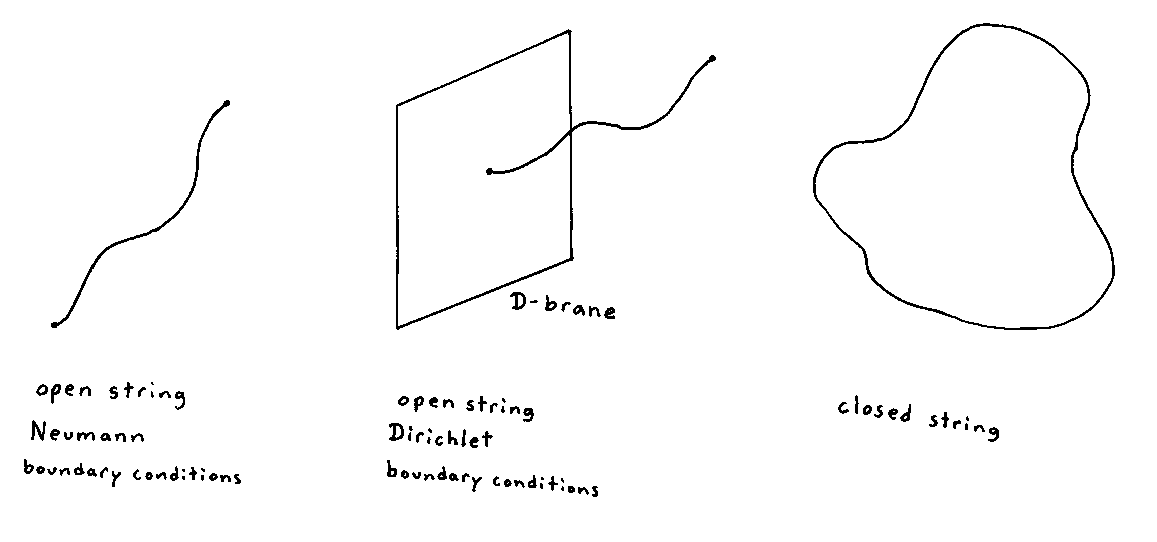
For a closed string, by convention, the spatial coordinate changes by π as you go around the string once. Therefore, you have

x^u ([sigma], [tau]) = x^u ([sigma] + [pi], [tau])

For an open string, which has two ends, each end is required to satisfy either Neumann or Dirchlet boundary conditions, for each value of u.

Neumann boundary conditions

[partial derivative of x^u with respect to [sigma]] = 0

for each end, meaning for when σ = 0 or π

Dirichlet boundary conditions

[partial derivative of x^u with respect to [tau]] = 0

for each end, meaning for when σ = 0 or π

The Dirichlet condition can be integrated, and then it specifies a spacetime location on which a string ends. Today, most people think of open strings as always ending on D-branes, so for Neumann boundary conditions, people imagine the string ending on a D-brane that fills all of space, so the string end can be located anywhere.

For a closed string, the general solution of the two-dimensional wave equation is given by a sum of the right-movers and left-movers. If waves on a closed string are propagating clockwise, that’s called a right-mover, and is represented by

x_R^u ([tau] – [sigma])

If waves on a closed string propagate counterclockwise, that’s called a left-mover, and is represented by

x_L^u ([tau] + [sigma])

The general solution is the sum of them, which is

x^u ([sigma], [tau]) = x_R^u ([tau] – [sigma]) + x_L^u ([tau] + [sigma])

These are subject to the following additional constraints.

x^u ([sigma], [tau])

is real

x^u ([sigma] + [pi], [tau]) = x^u ([sigma], [tau])

and

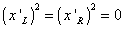
(x’_L)² = (x’_R)² = 0

These are called the T_{α β} = 0 constraints. The first two of the three conditions can be solved using a Fourier series.

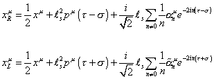
x_R^u = (1/2) x^u + l_s² p^u ([tau] – [sigma]) + (i/[squarerooot of 2]) l_s [summation over n which is not 0] (1/n) [alpha]_n^u e^{-2in([tau] – [sigma])}

x_L^u = (1/2) x^u + l_s² p^u ([tau] + [sigma]) + (i/[squarerooot of 2]) l_s [summation over n which is not 0] (1/n) [alpha tilda]_n^u e^{-2in([tau] + [sigma])}

where the expansion parameters satisfy

[alpha]_-n^u = ([alpha]_n^u)^†

[alpha tilda]_-n^u = ([alpha tilda]_n^u)^†

The center of mass coordinate x^u, and the momentum p^u are real. The fundamental string length scale l_s is related to the tension T by

T = (1/2[pi] [alpha]’)

[alpha]’ =l_s²

The parameter α’ is called the universal Regge slope. This harkens back to the old Regge theory. The string modes lie on linear parallel Regge trajectories with this slope.

Next we set up the commutation relations to quantize the string. It’s the same for closed string left-mover modes, closed string right-mover modes, and open string modes, so we’ll just look at the closed string right-movers. Using the gauge-fixing action, the canonical momentum of the string is

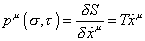
p^u ([sigma], [tau]) = [partial derivative of S with respect to [x dot]] = T [x dot]^u

Canonical quantization, which is just the tree level 2D field theory for scalar fields, gives

[p^u ([sigma], [tau]), x^v ([sigma]’, [tau])] = i[h bar] n^uv [delta] ([sigma] – [sigma]’)

In order to quantize the string, it must obey the following commutation relations. Using Fourier modes

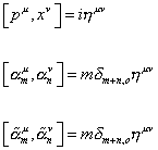
[p^u, x^v] = in^uv

[[alpha]_m^u, [alpha]_n^v] = m[delta]_{m + n, o} n^uv

[[alpha tilda]_m^u, [alpha tilda]_n^v] = m[delta]_{m + n, o} n^uv

and all other commutators vanish. Note that α_-m^u are like creation and annihilation operators. When you consider operators, you should write them in normal ordered form, where the creation operators are on the left, and annihilation operators are on the right. A quantum mechanic harmonic oscillator can be described in terms of raising and lowering operators, called a^† and a, which satisfy

[a, a^†] = 1

You can see that aside from a normalization factor, the expansion coefficients α_-m^u and α_m^u are raising and lowering operators. You might have noticed that because

n⁰⁰ = -1

the time components are proportional to oscillators with the wrong sign. This could lead to negative probabilities. However, the T_{α β} = 0 constraints eliminate the negative norm states from the physical spectrum.

Now, a closed string is like a circle, so let’s take the group of diffeomorphisms of the unit circle, and take it’s Lie algebra. That Lie algebra is called the Virasoro algebra. In string theory, you commonly use the Virasoro algebra which is defined as

[L_m, L_n] = (m – n) L_{m + n}

It becomes anomalous once quantum corrections are included, leading to the Virasoro algebra with central charges

[L_m, L_n] = (m – n) L_{m + n} + (c/12) (m³ – m) [delta]_{m + n, o}

The second term is called the conformal anomaly term, and the constant c is called the central charge. The generators L_n of the coordinate transformations are related to moments of the two-dimensional energy-momentum tensor T₀₀ – T₁₁ and T₀₁, which vanish due to the gauge-fixing equation.

Another thing you can do is take the group of maps from the unit circle to an arbitrary Lie group. That is called a loop group. Then take the Lie algebra of the loop group, and you get a Lie algebra called the Kac-Moody algebra, which is also used in string theory.

The following defines the Virasoro operators.

L_m = (T/2) [integral from 0 to [pi]] e^-2im[sigma] (x’_R) d[sigma] = (1/2) [summation over n from -infinity to infinity] [alpha]_{m – n} . [alpha]_n

Since α_m^u does commute with α_-m^u, you have to define L₀

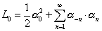
L₀ = (1/2) [alpha]₀² + [summation over n] [alpha]_-n . [alpha]_n

where

[alpha] = (l_s p^u)/[square root of 2]

and p^u is the momentum.

The following complex vector space is an inner product space

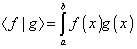
< f | g > = [integral from a to b] f(x) g(x)

This inner product gives us a positive definite norm for each vector

|| f || = [square root of < f | f >]

A Hilbert space is an inner product space which, as a metric, is complete. The Hilbert space of a harmonic oscillator is spanned by states | n >, n = 0, 1, 2, …where the ground state | 0 > is annihilated by the operator

a | 0 > = 0

and

| n > = ((a^†)ⁿ/[square root of n!]) | 0 >

Then for a normalized ground state

< 0 | 0 > =1

You can use [a^†, a] = 1 repeatedly to prove that

< m | n > = [delta]_{m, n}

and

a^† a | n > = n | n >

The string spectrum of right-movers is given by the product of an infinite number of harmonic oscillator Fock spaces, one for each α_n^u, subject to the Virasoro constraints

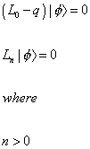
(L₀ – q) | [phi] > = 0

L_n | [phi] > = 0, n > 0

where | φ > is the physical state, and q is a constant. It accounts for the arbitrariness in the normal ordering prescription used to define L₀. The L₀ equation is a generalization of the Klein-Gordon equation. It contains

p² = -[partial derivative] . [partial derivative]

and oscillator terms whose eigenvalue will determine the mass of the state. You have to set the parameter q = 1 so that the mass shell condition becomes

(L₀ – 1) | [phi] > = 0

The mathematics of the open string spectrum is the same as the closed string right-movers, so let’s use the equations we just obtained to look at the open string spectrum. Here we are assuming all boundary conditions are Neumann, in other words, the D-branes they are attached to fill all of space. The mass shell condition is

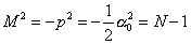
M² = -p² = -½ [alpha]₀² = N – 1

where p is the momentum, and

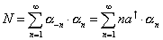
N = [summation over n from 1 to infinity] [alpha]_-n . [alpha]_n = [summation from n from 1 to infinity] na^† . a_n

where the a^†‘s and a’s are properly normalized creation and annihilation operators. Since a^† a has eigenvalues 0, 1, 2, …, the possible values of N are also 0, 1, 2, … You have N = 0 if all the oscillators are in the ground state. Now look at the following equation.

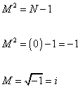
M² = N – 1

M² = (0) – 1 = -1

M = [square root of -1] = i

The first particle will then have imaginary mass, which we assume is impossible. In fact, this is another manifestation of the vacuum energy or zero point energy. Remember in my paper on the Standard Model in the section on electromagnetism, and more recently in this paper, in the section on supersymmetry, I gave the following relation for the energy of a particle system.

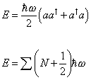
E = ([h bar]w/2) (aa^† + a^† a)

E = [summation] (N + ½) [h bar]w

When N = 0, the energy is more than zero, meaning the vacuum has energy. Here we are seeing a similar thing again. In this case, it predicts a particle with imaginary mass. What do you call a particle with imaginary mass? It’s called a tachyon, which was first theorized by Gerald Feinberg in 1967. If you look at the equation for the Lorentz factor γ, where γ = 1/[squareroot of (1 – (v/c)²)], you will see that if v > c, then γ is imaginary. From that you get imaginary mass. The tachyon has become immensely popular with science-fiction writers because it’s supposed to be a particle that travels faster than light. In a certain sense, that’s true, but it does not violate special relativity because it would not be possible to use a tachyon to send a message faster than light. Either localized disturbances in the wave equations do not propagate faster than light, or if the waves do seem to move faster than light, the waves are never localized in the first place. Therefore, even if tachyons were to exist, they could not be used to send a message faster than light, so they would not violate special relativity.

It’s reminiscent of the so-called EPR paradox in quantum mechanics, where if experiments violate the Bell Inequality, and in a certain sense, a particle could be said to instantly effect a distant particle, it would still not be possible for a person to use this to send a message to another person faster than light. Therefore, it does not violate special relativity.

However, despite its consistency with special relativity, the tachyon is still considered impossible. If they accelerate, they lose energy. A zero-energy tachyon would be infinitely fast. Since a tachyon moves faster than the speed of light in vacuum, it would produce Cerenkov radiation just be traveling though vacuum. Converting part of their radiation to energy, would lower their energy, causing them to accelerate more. Accelerating more would cause them to produce even more energy. You would have a run away reaction, where a tachyon ended up producing an infinite amount of energy, in the form of Cerenkov radiation, out of nothing. If tachyons existed, the vacuum would have to produce tachyon-antitachyon pairs all the time, each of which would undergo this run away effect. Throughout all of space, there would be an infinite number of tachyons, each of which would create an infinite amount of energy out of nothing. The Universe would exist at some sort of infinite energy scale, whereas the Planck scale is considered the highest energy scale possible in the real Universe. Obviously, this is not the Universe we live in. Any theory that predicts a tachyon is a flawed theory. Thus, the string theory we’ve been discussing so far, the bosonic string, is a flawed theory. However, like I said earlier, supersymmetry can cause the bosonic and fermionic contributions to the vacuum energy to cancel each other out, and leave no vacuum energy. I said that the problem of the tachyon is related to the problem of the vacuum energy, so supersymmetry solves the problem. Therefore, in superstring theory, there is no tachyon.

The ground state of the open string spectrum is

| [phi] > = 0

This gives N = 0, and M² = 1, or M = i, which is the tachyon, proving that the bosonic string is not a realistic theory. The first excited state in the open string spectrum is

| [phi] > = [zeta]_u [alpha]_-1^u | 0 >

where ζ_u is the polarization vector of a massless spin-1 particle. This gives N = 1, and M² = 0, or M = 0. The Virosoro constraint

L₁ | [phi] > = 0

implies ζ_u must satisfy

p^u [zeta]_u = 0

In four spacetime dimensions, a massless particle has two transverse polarization states. More generally, in d dimensions, a massless particle has d – 2 transverse polarization states. One of the dimensions is time. Another one of the dimensions is the longitudinal direction. The rest are transverse polarization states.

The second excited state in the open string spectrum is

| [phi] > = ([zeta]_u [alpha]_-2^u + [lambda]_uv [alpha]_-1^u [alpha]_-1^v) | 0 >

This corresponds to N = 2, and M² = 1, or M = 1. The Virasoro constraint

L₁ | [phi] > = L₂ | [phi] >

restricts ζ_u and λ_uv. When d = 26, this state becomes zero norm, and decouples from the theory. This leaves a massive spin-2 particle. There’s no such particle in real life. The only spin-2 particle is the graviton, which is massless. However, the fact it predicts a spin-2 particle of any type is a sign we’re on the right track.

Next, we’ll look at the closed string spectrum. You have both left-movers and right-movers, each of which are the same as the open string states. Therefore, a closed string state is described by a tensor product of a left-moving state and a right-moving state, subject to the condition that the N value of the left-moving state and the right-moving state are the same. The reason for this level matching condition is that we have

(L₀ – 1) | [phi] > = ([L tilda]₀ – 1) | [phi] > = 0

The left-movers and right-movers are distinguished by showing a tilda over the right-movers, probably because in heterotic string theories, the right-movers are supersymmetric, although in this case, neither is supersymmetric. The sum

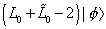
(L₀ + [L tilda]₀ – 2) | [phi] >

is interpreted as the mass shell condition, while the difference

(L₀ – [L tilda]₀) | [phi] > = (N – [N tilda]) | [phi] > = 0

is the level matching condition. The closed string states are the tensor product of the left-movers and right-movers. Therefore, the closed string ground state is

| 0 > x | 0 >

which is a spin-0 tachyon with M² = -2. Again, this means you have an unstable vacuum. The first excited state is

| [phi] > = [zeta]_uv ([alpha]_-1^u | 0> x [alpha]_-1^v | 0 >)

which has M² = 0. The Virasoro constraints

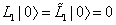
L₁ | [phi] > = [L tilda]₁ | [phi] > = 0

imply that

p^u [zeta]_uv = 0

This polarization tensor encodes three distinct spin states, each of which has a fundamental role in string theory. The symmetric part of ζ_uv encodes a spacetime metric field g_uv, corresponding to a massless spin-2 particle, and a scalar field φ, corresponding to a massless spin-0 particle. The spin-2 particle is the graviton. The spin-0 particle is the dilaton. The g_uv field means that the theory contains general relativity to a good approximation for

E << 1/l_s

where l_s is the string length. It’s vacuum value determines the spacetime geometry. The value of the dilaton field φ determines the string coupling constant.

g_s = e^[phi]

ζ_uv also has an antisymmetric part, which corresponds to a massless antisymmetric tensor gauge field, called the Kalb-Ramond field. B_uv = -B_uv It can be viewed as analogous to an electromagnetic field. In electromagnetism, you have the gauge transformation rule for the electromagnetic field.

[delta]A_u = [partial derivative]_u [capital lambda]

You have the gauge-invariant field strength.

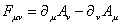
F_uv = [partial derivative]_u A_v – [partial derivative]_v A_u

A charged particle is a source of a vector potential A_u. The coupling of a charged particle to an electric field is

q [integral] A_u dx^u

and this means that the lightest charged particle, the electron, is stable. Similarly, the B_uv field has a gauge transformation of the form

[delta]B_uv = [partial derivative]_u [capital lambda]_v – [partial derivative]_v [capital lambda]_u

The gauge invariant field strength is

H_uvp = [partial derivative]_u B_vp + [partial derivative]_v B_pu + [partial derivative]_p B_uv

The fundamental string is a source for the B_uv field. This is expressed by the coupling.

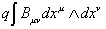
q [integral] B_uv dx^u [wedge product]dx^v

and this means that strings, which are charged under this field, are stable.

The number of physical states is given by

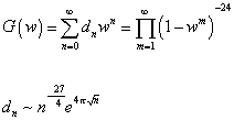
G(w) = [summation over n] d_n wⁿ = [product series over m] (1 – w^m)^-24

d_n ~ n^(-27/4) e^{(4[pi] [square root of n])}

where G(w) is the generating function, and d_n is the number of states, and the exponent 24 reflects the fact that in 26 dimensions, there are 24 polarized states.

Perturbation theory calculations are done by computing Feynman diagrams. In ordinary particle physics, the Feynman diagrams are networks of world lines. In string theory, they are two-dimensional surfaces, which are the world sheets of strings. We assume the world sheet metric h_{α β} is positive definite so the geometry is Euclidean. The diagrams are classified by their topology. With point particles, successively higher terms in the perturbative expansion correspond to an increasing number of internal loops in the Feynman diagrams. With string world sheets or tubes, these correspond to handles. Therefore, the higher the number of terms included in the perturbative expansion, the higher the genus of the manifold that is the world sheet that comprises the Feynman diagram. The Euler characteristic of a manifold is given by

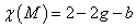
X(M) = 2 – 2g – b

or

X(M) = 2 – 2h – b

where g or h is the genus or number of handles, and b is the number of boundaries. A sphere has no handles and no boundaries, so g = b = 0, and χ = 2 – 2(0) – (0) = 2. A torus has one handle and no boundaries, so g = 1, b = 0, and χ = 2 – 2(1) – (0) = 0. A finite cylinder has two boundaries and no handles, so g = 0, b = 2, and χ = 2 – 2(0) – (2) = 0. A Klein bottle also has a Euler characteristic of 0. Surfaces with χ = 0 admit a flat metric. The order of the expansion, meaning the power of the string coupling constant, is determined by the Euler number of the world sheet.

Leonard Euler (1707 – 1783) came up with many equations or formulas now named after him, and one them stated that if you take any polyhedron, the number of vertices minus the number of edges plus the number of faces is always two. Here are versions of Euler’s formula in 1 – 4 dimensions.

1D → V = 2

2D → V – E = 0

3D → V – E + F = 2

4D → V – E + F – C = 0

where V is vertices, E is edges, F is faces, and C is cells, which are the 3D “faces” of 4D polytopes. So there is a pattern, where with each additional dimension, you add an additional term to Euler’s formula, and the sign of the additional terms alternates minus, plus, minus, etc., and the “answer” of the formula alternates 2, 0, 2, 0, etc. This pattern continues for higher dimensions. The reason for the number two is because polygons, polyhedra, and polytopes are circumscribed within the manifold Sⁿ which has an Euler characteristic of two.

In algebraic topology, the Euler characteristic of a space is the alternating sum of the “ranks of the its rational homology groups”, and you can compute these using any way of chopping up the space into convex polytopes. Some spaces have an ill-defined Euler characteristic because they either have infinitely many nonzero rational homology groups, typical of infinite-dimensional spaces, or rational homology groups of infinite rank, such as an infinite genus torus. Compact manifolds don’t have these problems. Of course, the Euler characteristic is defined for many spaces other than compact manifolds.

A scattering amplitude is given by the path integral

[integral] Dh_{[alpha] [beta]} ([sigma]) Dx^u ([sigma]) e^{-S[x, h]} [product series over i to n_c] V_[alpha]i ([sigma]_i) d² [sigma]_i [product series over j to n_o] V_[beta]j ([sigma]_j) d² [sigma]_j

where

S[x, h] = -(T/2) d² [sigma] [square root of -h] h^{[alpha] [beta]} n_{[alpha] [beta]} [partial derivative]_[alpha] x^u [partial derivative]_[beta] x^v

and where n_c is the number of closed strings, n_o is the number of open strings, V_αi is a vertex operator that describes emission or absorbtion of a closed string of type α_i from the interior of the string world sheet, and V_βj is a vertex operator that describes emission or absorbtion of an open string of type β_j from the boundary of the string world sheet. The conformally inequivalent world sheets of a given topology are described by a finite number of parameters. Therefore, these amplitudes can be written as finite-dimensional integrals over these moduli. The dimension of the resulting integral is

N = 3(3g + b – 2) + 2n_c + n_o

The following defines the Euler beta function.

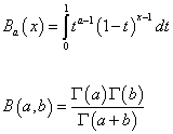
The scattering amplitude is given by

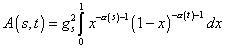
A(s, t) = g_s² [integral from 0 to 1] x^{-[alpha](s) – 1} (1 – x)^{-[alpha](t) – 1}dx

where the Mandelstam invariants s and t, and the Regge trajectory α(s) are given by

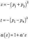
s = -(p₁ + p₂)²

t = -(p₁ – p₄)²

[alpha](s) = 1 + [alpha]’s

Mandelstam variables are Lorentz-invariant variables describing the kinematics of particle reactions. Originally the variables were introduced by Mandelstam to describe two-body elastic scattering amplitudes in terms of dispersion relations as functions of two complex variables s and t. Mandelstam variables are also widely used now to describe the kinematics of multibody final states viewed as two incident and two outgoing systems.

Using the Euler beta function, you have

A(s, t) = g_s² B(-[alpha](s), -[alpha](t)) = g_s² (([capital gamma](-[alpha](s)) [capital gamma] (-[alpha](t)))/([capital gamma] (-[alpha](s) – [alpha](t))))

This is called the Veneziano amplitude.

The bosonic string is the first renormalizable theory of gravity, which is a great achievement. However, it is obviously a seriously flawed unrealistic theory. First of all, it contains only bosons with no fermions at all. Second of all, it includes the tachyon. Fortunately, both of these problems can be solved by combining string theory with supersymmetry, resulting in superstring theory. In supersymmetry, you add anticommutators which give rise to fermions. The bosons end up with supersymmetric partners which are fermions, so that way you can get fermions. Also in supersymmetry, the bosonic contributions to the vacuum energy are canceled out by fermionic contributions of identical magnitude and opposite sign. This mechanism is used to cancel out the self-energy contributions to the Higgs mass. As I described, this vacuum energy is the origin of the tachyon. Therefore, supersymmetry allows you to get rid of the tachyon. Therefore, superstring theory contains both bosons and fermions, and no tachyon. An additional benefit of superstring theory is that it reduces the number of dimensions from 26 to 10, so you have fewer extra dimensions to compactify.

As I said before, the following is the Virasoro algebra.

[L_n, L_m] = (n – m)L_{n + m}

The following is the Virasoro algebra with central charges.

[L_n, L_m] = (n – m)L_{n + m} + (c/12) (m³ – m) [delta]_{m + n, o}

where the second term is the conformal anomaly term, and c is the central charge. The theory has conformal invariance.

In 1971, Pierre Ramond studied solutions to the Dirac equation of the string world sheet. This led to a much larger symmetry algebra than the Virasoro algebra. This new algebra included anticommutating operators, F_n, analogous to the supersymmetry generators Q. This modified Virasoro algebra is

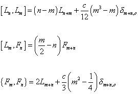
[L_n, L_m] = (n – m)L_{n + m}

[L_m, F_n] = ((m/2) – n) F_{m + n}

{F_m, F_n} = 2L_{m + n} + (c/3) (m² – (1/4)) [delta]_{m + n, o}

This is called the super-Virasoro algebra. This algebra has superconformal invariance.

Also in 1971, John Schwarz and Andre Neveu worked on a bosonic string theory that had an anticommuting field with half integer boundary conditions on the world sheet. They also found a super-Virasoro algebra, although it was slightly different from Ramond’s version. Gervais and Sakita determined that the two theories developed by Ramond and by Neveu and Schwarz fit together into two sectors of the same theory, called the RNS formalism. Historically, it was also called the spinning string theory. In this formalism, the supersymmetry is on the two-dimensional world sheet as it propagates through spacetime. A different formalism, developed by Michael Green and John Schwarz in 1981, has the supersymmetry on the 10-dimensional spacetime itself. The second formalism, called the GS formalism, removed any doubt as to whether superstring theory was truly supersymmetric in the traditional sense, and greatly improved the standing and popularity of superstring theory.

In the non-supersymmetric case, you had the following function that describes the world sheet.

x^u ([sigma], [tau])

where σ parametrizes the position of a point on the string, and τ gives the time evolution. In addition to that, in the supersymmetric case, you also have fermionic partner fields.

[psi]^u ([sigma], [tau])

x^u transforms as a vector from the 10-dimensional spacetime point of view, and as d scalar fields from the two-dimensional world sheet point of view. ψ^u transforms as a vector from the spacetime point of view, and as a spinor from the world sheet point of view. Together, x^u and ψ^u describe d supersymmetry multiplets, one for each value of u, where u = 0, 1, …d-1, and d is the dimensionality of spacetime.

When you choose a suitable conformal gauge

h_{[alpha] [beta]} = e^[phi] n_{[alpha] [beta]}

plus an appropriate fermionic condition, you end up with a world sheet theory that has global supersymmetry with constraints. The constraints form a super-Virasoro algebra. Therefore, in addition to the Virasoro constraints on the bosonic string theory, there are also fermionic constraints.

Remember that for the bosonic string, you had the gauge-fixed action.

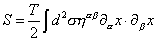
S = (T/2) [integral] d² n^{[alpha] [beta]} [partial derivative]_[alpha] x . [partial derivative]_[beta] x

where T is the tension, and η_{α β} is the two-dimensional Minkowski metric of the flat world sheet. The globally supersymmetric world sheet action that arises in the conformal gauge is

S = -(T/2) [integral] d² [sigma] ([partial derivative]_[alpha] x^u [partial derivative]^[alpha] x_u -i[psi bar]^u p^[alpha] [partial derivative]_[alpha] [psi]_u)

The first term is the same as the bosonic string case, which has the structure of d free scalar fields. The second term is d free massless spinor fields. p^α is two 2 x 2 Dirac matrices, and

is a two-component Majorana spinor.

∂₊

is the derivative with respect to

[sigma]⁺ = [tau] + [sigma]

and ∂_–

is the derivative with respect to

[sigma]^– = [tau] – [sigma]

The Majorana condition means that ψ₊ and ψ_– are real in the representation of the Dirac algebra, which is

[psi bar] p^[alpha] [partial derivative][alpha] [psi] = [psi]_– [partial derivative]₊ [psi]_– + [psi]₊ [partial derivative]_– [psi]₊

The equations of motion are

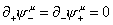
[partial derivative]₊ [psi]_–^u = [partial derivative]_– [psi]₊^u = 0

Therefore, ψ_–^u describes right-movers, and ψ₊^u describes left-movers.

Let’s look at the right-movers. The global supersymmetry transformations, which are a symmetry of the gauge-fixed action, are

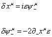
[delta]x^u = i[epsilon] [psi]_–^u

[delta][psi]_–^u = -2[partial derivative]_– x^u [epsilon]

The Virasoro constraint is

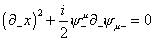
([partial derivative]_– x)² + (i/2) [psi]_–^u [partial derivative]_– [psi]_u- = 0

The first term is the same as for the bosonic string. The second term is an additional fermionic contribution. There is also the fermionic constraint

[psi]_–^u [partial derivative]_– x_u = 0

The Fourier modes of these constraints satisfy the super-Virasoro algebra. It’s the same for the left-movers.

Let’s look at the boundary conditions. The boundary conditions for the bosonic part

x^u ([sigma], [tau])

are exactly the same as what we did before for the bosonic string, so let’s look at the fermionic part

[psi]^u ([sigma], [tau])

You have ψ₊ which describes the left-movers, and ψ_– which describes the right-movers. Now at each end of the open string, the left-movers and right-movers could either be the same, or they could differ by a sign. In other words, you have

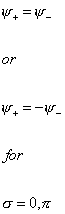
[psi]₊ = [psi]_–

or

[psi]₊ = -[psi]_–

for

[sigma] = 0, [pi]

Let’s say that they are the same at the end of the open string we’re calling 0. If they are the same at the 0 end of the open string, you have

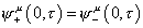
[psi]₊^u (0, [tau]) = [psi]_–^u = (0, [tau])

So at one end of the string, they are the same. Therefore, at the other end, which we call π, they are either the same, or of opposite sign. Therefore, you have two possibilities.

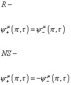
R-

[psi]₊^u ([pi], [tau]) = [psi]_–^u ([pi], [tau])

NS-

[psi]₊^u ([pi], [tau]) = -[psi]_–^u ([pi], [tau])

The first of the above two possibilities is called the Ramond boundary condition, or R. The second possibility is called the Neveu-Schwarz boundary condition, or NS. Sometimes, people call them the Ramond string and the Neveu-Schwarz string. The Ramond string is said to be periodic, and the Neveu-Schwarz string is said to be anti-periodic.

Remember the following equations of motion.

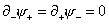
[partial derivative]_– [psi]₊ = [partial derivative]₊ [psi]_– = 0

This allows you to express the general solutions of the boundary conditions as a Fourier series.

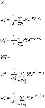
R-

[psi]_–^u = (1/[squareroot of 2]) [summation of n = Z] d_n^u e^{-in([tau] – [sigma])}

[psi]₊^u = (1/[squareroot of 2]) [summation of n = Z] d_n^u e^{-in([tau] + [sigma])}

NS-

[psi]_–^u = (1/[squareroot of 2]) [summation of n = Z + ½ ] b_n^u e^{-in([tau] – [sigma])}

[psi]₊^u = (1/[squareroot of 2]) [summation of n = Z + ½ ] b_n^u e^{-in([tau] + [sigma])}

The Majorana condition implies that

d_-n^u = d_n^u†

b_-r^u = b_r^u†

The index n only has integer values. The index r only has half-integer values. Only the R boundary condition gives a zero mode. You have the following anticommutation relations for the coefficients d_m^u and b_r^u.

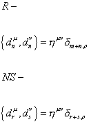
R-

{d_n^u, d_n^v} = [eta]^uv [delta]_{m + n, o}

m, n are contained in Z

NS-

{d_r^u, d_s^v} = [eta]^uv [delta]_{r + s, o}

m, n are contained in Z + ½

Therefore, in addition to the harmonic oscillator operators α_n^u that appear as coefficients in mode expansions of x^u, you also have fermionic oscillator operators d_n^u and b_r^u that appear in mode expansions of ψ^u.

The basic structure {b, b^†} = 1 describes a two-state system with b | 0 > = 0 and b^† | 0 > = | 1>. The b’s and d’s with negative indices are raising operators, and those with positive indices are lowering operators. It’s basically the same as what we did before for α_n^u.

All the states obtained by acting with the α and b raising operators are bosons. In a simple generalization of the bosonic string, in the NS sector, the ground state satisfies

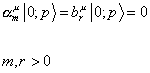
[alpha]_m^u | 0 ; p> = b_r^u | 0 ; p> = 0

m, r > 0

In the R sector, there are zero modes that satisfy the algebra

{d₀^u, d₀^v} = [eta]^uv

This is the d-dimensional spacetime Dirac algebra. The d₀‘s can then be regarded as Dirac matrices, and all the states in R are spinors. Therefore, all the string states in the NS sector are bosons, and all the string states in the R sector are fermions.

This was the case for the open string. With the closed string, you have both right and left movers at the same time. You have the product of the right and left movers, each of which is the same as the open string spectrum. Therefore, you have four separate sectors in the closed string states. If both the right-movers and left-movers have the same boundary conditions, meaning you have NS x NS or R x R, you have bosons. If they have different boundary conditions, meaning you have NS x R or R x NS, you have fermions.

The zero mode of the fermionic constraint

[psi]^u [partial derivative]_– x_u = 0

gives a wave equation for the fermionic strings in the Ramond sector

F₀ | [psi] > = 0

called Dirac-Ramond equation, where

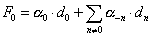
F₀ = [alpha]₀ . d₀ + [summation where n is not 0] [alpha]_-n . d_n

The fermionic ground state | ψ₀ > which satisfies

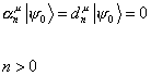
[alpha]_n^u | [psi]₀ > = d_n^u > = 0

n > 0

satisfies the wave equation

[alpha]₀ . d₀ | [psi]₀ > = 0

The action for the string in the conformal gauge is

S = T [integral] d[xi]⁰ d[xi]¹ ([partial derivative]^[alpha] x^u [partial derivative]_[alpha] x_u + [psi]^u [gamma]⁰ [gamma]^[alpha] [partial derivative]_[alpha] [psi] _n)

where α = 0, 1 are the world sheet coordinates, and ψ^u are two-dimensional Hermitian forms. The γ’s are given by

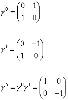
using

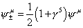
[psi]_±^u = ½ (1 + [gamma]⁵) [psi]^u

the fermionic part of the Lagrangian can be written as

L_F = [psi]₊^u [psi]_u+ + [psi]_–^u [partial derivative]₊ [psi]_u-

The field equations that follow from L_F are

[partial derivative]_-/+ [psi]_±^u = 0

ψ₊ is only a function of ξ₊, and ψ_– is a function of ξ_–. The Fourier expansion of ψ_±^u is

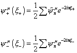
[psi]₊^u ([xi]₊) = ½ [summation] [psi tilda]_n^u e^-2in[xi]₊

[psi]_–^u ([xi]₊) = ½ [summation] [psi]_n^u e^-2in[xi]_–

For the Ramond string, n takes integer values, and for the Neveu-Schwarz string, n takes half-integer values. Therefore, for the NS case, you have

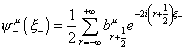
[psi]_–^u ([xi]_–) = ½ [summation of r from -infinity to infinity] b_{r + ½}^u e^{-2i (r + ½)[xi]_–}

and in the R case, you have

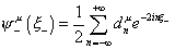
[psi]_–^u ([xi]_–) = ½ [summation of n from -infinity to infinity] d_n e^-2in[xi]_–

Now, let’s look at the vacuum state | 0 >, the one particle state b_{– ½} | 0>, etc. where it goes over d – 2 transverse dimensions, with i = 2, 3, …d – 1. For the Ramond string, you have

{d₀^u, d₀^v} = [eta]^uv

This is the Clifford algebra, and has a 2^d/2 dimensional representation in the ground state. Therefore, the ground state must transform as a spinor representation of the Lorentz group. Only the fermions transform according the spinor representation of the Lorentz group. Therefore, the Ramond string must lead to fermions, unlike the bosonic string or the Neveu-Schwarz string which lead to bosons.

Now let’s evaluate the world sheet energy-momentum tensor T_αβ, and obtain its Fourier coefficients.

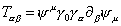
T_{[alpha][beta]} = [psi]^u [gamma]₀ [gamma]_[alpha] [partial derivative]_[beta] [psi]_u

From this you get

T₊₊ = [psi]₊ [partial derivative]₊ [psi]₊

T_— = [psi]_– [partial derivative]₊ [psi]_–

The fermionic contribution to L₀ for NS is

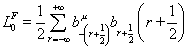
L₀^F = ½ [summation over r from -infinity to infinity] b_{-(r + ½)}^u b_{r + ½} (r + ½)

and for R is

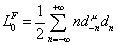
L₀^F = ½ [summation over n from-infinity to infinity] nd_-n^u d_n

The vacuum energy for the Neveu-Schwarz case is

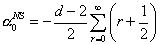
[alpha]₀^NS = -((d – 2)/2) [summation over r from 0 to infinity] (r + ½)

The first excited state is

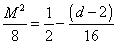
M²/8 = ½ – (d – 2)/16

Since there are not enough components of this state to form an irreducible representation of the SO(d – 2) group, this state must have zero mass. So if M = 0, then d = 10.

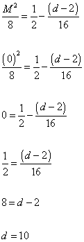
M²/8 = ½ – (d – 2)/16

( 0 )²/8 = ½ – (d – 2)/16

0 = ½ – (d – 2)/16

½ = (d – 2)/16

8 = d – 2

d = 10

Therefore, the inclusion of Neveu-Schwarz string reduces the critical dimension from 26 to 10. Therefore, superstrings exist in ten spacetime dimensions.

You have the total number of spacetime dimensions. One of the dimensions is time. One is the longitudinal direction of a particle traveling through it. So for d = 4, which is normal spacetime, you have two transverse directions. The bosonic string requires d = 26, which has 24 transverse directions. Superstring theory requires d = 10, which has eight transverse directions.

With the bosonic string, you only had the α oscillators. Each α contributes -1/24 to the normal ordering constant, for each transverse direction. In the bosonic string, you have 24 transverse directions so

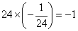
24 x (-1/24) = -1

so the bosonic string theory has a normal ordering constant of -1, and therefore has the mass formula

M² = N -1

With superstrings, you have both the α oscillators and the b oscillators. The α oscillators contribute -1/24 to the normal ordering constant, as before, and in addition, the b oscillators each contribute -1/48 to the normal ordering constant. In superstring theory, you have eight transverse directions so you have

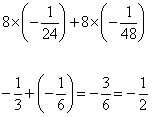
8 x (-1/24) + 8 x (-1/48)

-1/3 + (-1/6) = -3/6 = -1/2

so superstring theory has a normal ordering constant of -½, and therefore has the mass formula

M² = N – ½

To repeat, the mass formula for the bosonic string is

M² = N – 1

In the lowest state, N = 0, so you have

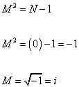
M² = ( 0 ) -1 = -1

M = [squareroot of -1] = i

so therefore you have a tachyon which is an impossible particle. The mass formula for the superstring is

M² = N – ½

In the lowest state, N = 0, so you have

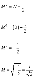
M² = ( 0 ) – ½

M² = -½

M = [squareroot of -½] = i/[squareroot of 2]

so you still have a tachyon which creates an unstable vacuum. Therefore, as of now, superstring theory still contains a tachyon in the spectrum. However, with superstring theory, there exists a way to get rid of it which did not exist for the bosonic string. This is achieved by using the GSO projection, which was developed by Ferdinando Gliozzi, Joel Sherk, and David Olive in 1976.

The GSO projection is a truncation in the NS sector, where you keep the states with an odd number of b oscillator excitations, and remove the states with an even number of b oscillator excitations. When you do this, N can take only half-integer values. The mass formula is the same

M² = N – ½

except now, the lowest value of N is not zero but ½. Therefore, you have

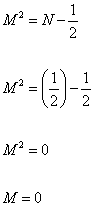
M² = ( ½ ) – ½

M² = 0

M = 0

Therefore, you don’t have a tachyon. You could not have done this with the bosonic string since there are no b oscillators to manipulate. The possible values for M² are

M² = 0, 1, 2,…

The GSO projection also acts on the R sector where there is an analogous restriction on the d oscillators. This imposes a chirality projection on the spinors.

Let’s look at the massless spectrum of the GSO projected theory. The ground state is a massless boson represented by the state

[zeta] b_-½^u | 0 ; p>

which has d – 2 = (10) – 2 = 8 physical polarizations. The ground state fermion is a massless Majorana-Weyl fermion which has 8 physical polarizations.

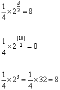
¼ x 2^d/2 = 8

¼ x 2^(10)/2 = 8

¼ x 2⁵ = ¼ x 32 = 32/4 = 8

Therefore, the ground state boson and the ground state fermion both have the same number of physical polarizations as required by a supersymmetry theory. You have equal numbers of bosons and fermions as required by a theory with spacetime supersymmetry. This is a pair of fields that enter into the 10-dimensional Yang-Mills theory. You have an equal number of bosons and fermions at every mass level. Therefore, the superstring theory has full spacetime supersymmetry.

For the bosonic string, the generating function is

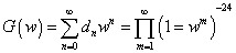
G(w) = [summation over n from 0 to infinity] d_n wⁿ = [product series over m from 1 to infinity] (1 – w^m)^-24

where d_n is the number of physical states with

[alpha]’ M² = n – 1

and

d_n ~ n^-27/4 e^{4[pi][squareroot of n]}

Let’s say d_NS ( n ) is the number of bosonic states with M² = n, and d_R ( n ) is the number of fermionic states with M² = n. Then the generating functions for the Neveu-Schwarz string and the Ramond string are

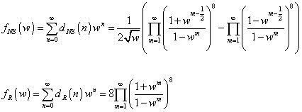
f_NS = [summation over n from 0 to infinity] d_NS (n) wⁿ = (1/(2[squareroot of w])) ([product series of m from 1 to infinity] ((1 + w^{m – ½})/(1 – w^m))² – [product series of m from 1 to infinity]((1-w^{m – ½})/(1 – w^m))⁸)

f_R = [summation over n from 0 to infinity] d_R (n) wⁿ = 8[product series of m from 1 to infinity]((1 + w^m)/(1 = w^m))⁸

The 8’s in the exponents refer to the number of transverse directions in ten dimensions. The GSO projection causes the subtraction of the second term in f_NS, and the reduction of the coefficient in f_R from 16 to 8.

Before using the GSO projection, the allowed states for the Neveu-Schwarz string include

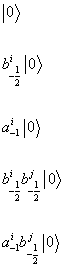
| 0 >

b_-½ⁱ | 0 >

a_-1ⁱ | 0 >

b_-½ⁱb_-½^j | 0>

a_-1ⁱb_-½ⁱ

| 0>

After using the GSO projection, the only allowed states are

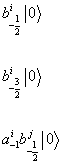
b_-½ | 0 >

b_-3/2ⁱ | 0 >

a_-1ⁱ b_-½^j | 0 >

For a closed string, all the points on the string are the same, and are therefore invariant under the shift

[sigma] -> [sigma] + [delta] [sigma]

The unitary operator for the shift is

U = e^{2i[delta][sigma](L₀ – [L tilda]₀)}

For it to be invariant, U = 1, which is only true if

L₀ = [L tilda]₀

which means the allowed energy levels are those for which the right-movers and left-movers have the same mass. The massless states are

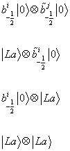
b_-½ⁱ | 0 > x [b tilda]_-½^j | 0>

| La > x [b tilda]_-½ | 0 > x | La >

| La > x | La >

The first one gives the graviton, h^ij = h^ij, the antisymmetric field, b^ij = -b^ji, and the dilaton, φ. The next two give rise to the gravitino and the dilatino. The last one gives rise to a set of 64 scalar bosons.

Now, let’s look at the five superstring theories, which are Type I, Type IIA, Type IIB, Heterotic SO(32), and Heterotic E₈ x E₈. Type I superstring theory has N = 1 supersymmetry, and therefore has 16 supercharges. It has unoriented closed and open strings. It is the only superstring theory with open strings. It has a Yang-Mills gauge group, which at the classical level, could be any SO(n) or Sp(n) group, for any value of n. However, when you take quantum effects into account, you have to choose a value for which the anomalies cancel. Quantum consistency requires that the gauge group be SO(32). For Type I superstrings, the SO(32) gauge quantum numbers are carried by the endpoints of the open strings. For the other string theories, the gauge quantum numbers are carried by the string itself. The SO(32) Yang-Mills gauge group is specifically on the open strings, so the spin-1 gauge bosons are on the open strings. The graviton is on the closed strings. Including both the open and closed strings, Type I superstring theory has spin-1 gauge bosons, the graviton, and fermions.

An n-dimensional spinor is an element of a specific projective representation of the rotation group SO(n, R), or more generally SO(p, q, R), where p + q = n for spinors in a space of nontrivial signature. This is equivalent to an ordinary non-projective representation of the universal cover of SO(p, q, R), which is a real Lie group called the spinor group Spin(p, q). The most common type of spinor is the Dirac spinor which is a member of the fundamental representation of the complexified Clifford algebra C(p, q), into which Spin(p, q) can be embedded. In even dimensions, this representation is reducible when taken as a representation of Spin(p, q), and can be decomposed into two representations called the left-handed and right-handed Weyl spinor representations. These are the same except for the actions of the parity transformation, which is not part of Spin(p, q) but is part of C(p, q). In addition, sometimes the non-complexified version of C(p, q) has a smaller representation called the Majorana spinor representation. In even dimensions, this can be decomposed into two representations called the left-handed and right-handed Majorana-Weyl spinor representations.

In the section on the bosonic string, I explained how the closed string states are the tensor product of the two open string states. You can do the same thing here, forming a closed string spectrum that is a tensor product of the two supersymmetric string states. Each consists of a vector and a Majorana-Weyl spinor. Therefore, you have a tensor product of a vector and a Majorana-Weyl spinor, and another vector and Majorana-Weyl spinor.

(vector + MW spinor) x (vector + MW spinor)

Now, the two spinors could have either same or opposite chirality. When the two spinors have opposite chirality, you have Type IIA superstring theory. When the two spinors have the same chirality, you have Type IIB superstring theory. With Type IIA superstring theory, the massless spectrum forms the Type IIA supergravity multiplets. Since the two spinors have opposite chirality, they cancel each other out. This means that the resulting theory is left-right symmetric, or parity conserving. Since the real world is parity violating, this was initially considered strong evidence against Type IIA superstring theory. However, later it was figured out how to induce parity violation through the compactification process. If the two MW spinors have the same chirality, they re-enforce each other. Therefore, Type IIB superstring theory is chiral, or parity-violating.

Type IIA and Type IIB superstring theory have a vector x spinor and spinor x vector which are the gauge fields for the local supersymmetry. From this, you get two gravitinos. In four spacetime dimensions, gravitinos are spin 3/2, although the situation is more complicated in 10 spacetime dimensions. Since the Type II string theories have two gravitinos, they therefore have N = 2 supersymmetry. The supersymmetry charges are Majorana-Weyl spinors, which have 16 components, so the Type II theories have 32 conserved supercharges. This is the same amount of supersymmetry as N = 8 supersymmetry in four spacetime dimensions. Type II strings are also related to a type of bosonic string called Type 0.

Now, there is what originally appeared to be a major drawback to Type IIA and Type IIB superstring theories. Although in the bosonic string theory, you have bosons on closed strings, with superstrings, the Yang-Mills gauge groups, and thus the gauge bosons are only on open strings. Since Type IIA and Type IIB string theories have only closed strings, the string states don’t give rise to bosons, except of course for the graviton which is intrinsic in all closed strings. Therefore, these theories, in their original simple form, have half-integer spin particles, which are the fermions, and a spin-2 particle, which is the graviton, but no spin-1 particles, such as the photon. Since there are no gauge bosons, there is no gauge symmetry at all. However, later it was figured out a way to compactify the extra dimensions in such a way so that the compactification process itself gives rise to gauge bosons, and fermions charged under gauge interactions. This is another example of how the extra dimensions of string theory turned out to be a blessing in disguise since in the process of compactifying the extra dimensions, you can get rid of many of the problems in string theory, and arrive at a much more realistic theory of nature.

However, when the Type IIA and Type IIB superstring theories were first discovered, or invented, it was thought that they only had fermions with no bosons. Meanwhile, the bosonic string theory had only bosons but no fermions. If you could only combine these two closed string theories together, you could get a closed string theory with both bosons and fermions. This is the motivation behind the two heterotic string theories developed by D. Gross, J. Harvey, E. Martinez, and R. Rohm in 1985. On a closed string, the left-movers and right-movers operate totally independently of each other. What if the left-movers were non-supersymmetric, and the right-movers were supersymmetric? Then you could get one closed string that gives rise to both gauge bosons and fermions, as well as the graviton. The most obvious difficulty in having both non-supersymmetric and supersymmetric states on the same string is that the non-supersymmetric states exist in 26 dimensions, and the supersymmetric states exist in 10 dimensions. The solution is to initially compactify the extra 16 dimensions of the left-mover states on a torus, so they will both have 10 dimensions. Later, you can compactify six of those ten dimensions on another manifold to give rise to the familiar four spacetime dimensions. When you compactify the 16 extra dimensions on a torus, it gives rise to a local internal symmetry group of rank 16. It turns out that there are only two consistent possibilities for this group which are SO(32), same as the SO(32) group of Type I string theory, and E₈ x E₈. Therefore, there are two heterotic string theories, which are Heterotic SO(32) and Heterotic E₈ x E₈.

The real world is parity violating, so you would want a theory that is parity violating, unlike the Type IIA string theory that is parity conserving. However, if your theory is parity violating, you have the problem of chiral anomalies. Chiral gauge theories can be inconsistent due to chiral anomalies. This happens when you have a quantum mechanical breakdown of the gauge symmetry due to certain one-loop Feynman diagrams. The trick then is to choose a theory where the chiral anomalies cancel each other out so you end up with no anomalies in the resulting theory. In four spacetime dimensions, the offending diagrams are triangles. This is called the Adler-Bell-Jackiw anomaly, discovered by Steve Adler, and independently by John Bell and Roman Jackiw.

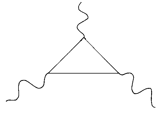
In the Standard Model, all of the chiral anomalies cancel each other out. In ten dimensional gauge fields, the anomalous Feynman diagrams are hexagons.

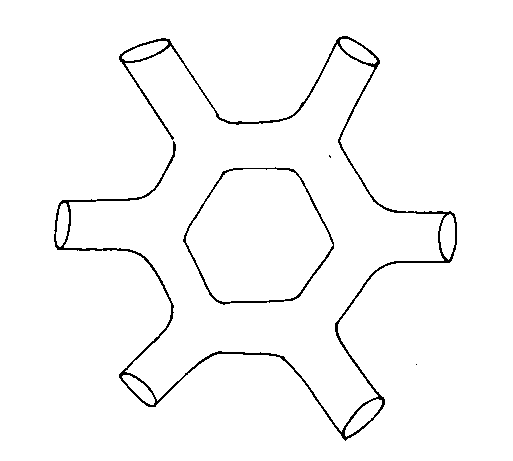
You should choose a theory in which the anomalies cancel each other out. Here are some possible theories.

1. N = 1 supersymmetric Yang Mills theory-

This is the theory for the open strings in Type I superstring theory. This theory has anomalies that do not cancel out.

2. Type I supergravity –

This is the theory for the closed strings in Type I superstring theory. This theory has anomalies that do not cancel out.

3. Type IIA supergravity –

This is the theory for Type IIA superstrings. Since the theory is non-chiral, it therefore can’t have chiral anomalies.

4. Type IIB supergravity –

This is the theory for Type IIB superstrings. This theory has three chiral fields, each of whom contribute anomalies. However, in 1983, Edward Witten and Alvarez-Gaume proved that all the anomalies cancel.

5. Type I supergravity coupled to supersymmetric Yang-Mills –

This is the theory of the two heterotic superstrings. This theory has anomalies for every choice of Yang-Mills gauge group except SO(32) and E₈ x E₈. The theory has anomalies but all the anomalies cancel if and only if the gauge group is either SO(32) or E₈ x E₈. This was proved by John Schwarz and Michael Green in 1984. This mechanism is called the Green-Schwarz anomaly cancellation mechanism.

Therefore, at one time, the two heterotic string theories really seemed to be our best hope, since in Type I string theory, the anomalies don’t cancel, and in Type IIA and Type IIB, there did not seem to be any spin-1 gauge bosons. The two Lie group SO(32) and E₈ x E₈ have several properties in common. They are both rank 16, and are 496-dimensional. Their weight lattices correspond to the only two even self-dual lattices in 16 dimensions. Remember that the heterotic strings have 26-dimensional left-movers, and 10-dimensional right-movers. The extra 16 dimensions of the left-movers are associated with an even self-dual 16-dimensional lattice. In this way, you can build in the SO(32) or E₈ x E₈ gauge symmetry.

The left-movers are bosonic, and thus have 26 dimensions, or 24 transverse directions, or 24 degrees of freedom. Of these, 16 are compactified coordinates. One bosonic degree of freedom is equivalent to two Majorana fermions. Therefore, the left-movers have 8 bosonic coordinates, and 32 fermionic coordinates. If all 32 fermions have the same boundary conditions, the gauge group will be SO(32). If 16 of the fermions have the same boundary conditions, you end up with E₈ x E₈.

For the SO(32) case, the states with zero mass are

[alpha tilda]_-1ⁱ | 0 >

[lambda tilda]_-½^A [lambda tilda]_-½^B | 0 >

The physical particle spectrum is

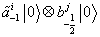
[alpha tilda]_-1ⁱ | 0 > x b_-½^j | 0 >

which is the graviton, h^ij, an antisymmetric field, b^ij, and the dilaton, φ

[alpha tilda]_-1ⁱ | 0 > x L

which is the gravitino and the dilatino

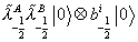
[lambda tilda]_-½^A [lambda tilda]_-½^B | 0 > x b_-½^j | 0 >

which is the gauge bosons

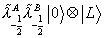
[lambda tilda]_-½^A [lambda tilda]_-½^B | 0 > x | L >

which is the gaugino.

The resulting low energy theory is a 10-dimensional N = 1 supergravity with an SO(32) Yang-Mills group.

For the E₈ x E₈ case, you have

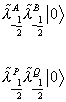
[lambda tilda]_-½^A [lambda]_-½ | 0 >

[lambda tilda]_-½^P [lambda tilda]_-½^Q | 0 >

The massless states are the Ramond vacuum which is a spinor under SO(16) which is 128-dimensional. This has two massless states. Adding these, you get in the A-sector, 120 + 128 = 248-dimensional representation, which is the adjoint representation of E₈. You have the same thing in the P-sector where you get another 248-dimensional representation of another E₈, leading E₈ x E₈ as the gauge group. Combining with the right-movers, you get a 10-dimensional N = 1 supergravity theory coupled with the E₈ x E₈ Yang-Mills group.

Here is the Lagrangian for the Heterotic E₈ x E₈ superstring theory.

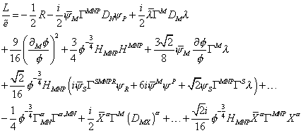
L/[e tilda] = -½R – (i/2) [psi bar]_m [capital gamma]^MNP D_N [psi]_P + (i/2) [lambda bar] [capital gamma]^M D_M [lambda] + (9/16) (([partial derivative]_M [phi])/[phi])² + (3/4) [phi]^-3/2 H_MND H^MND + (3[squareroot of 2]/8) [psi bar]_M (([partial derivative][phi])/[phi]) [capital gamma]^M [lambda] + ([squareroot of 2]/16) [phi]^-3/4 H_MNP (I[psi bar]_S [capital gamma]^SMNPR [psi]_R + 6i[psi bar]^M [psi]^P + [squareroot of 2] [psi]_S [capital gamma]^MNP [capital gamma]^S [lambda]) + …-¼[phi]^-3/4 [capital gamma]_MN^[alpha] [capital gamma]^{[alpha], MN} + i/2 [X bar]^[alpha] [capital gamma]^M (D_MX)^[alpha] + …+([squareroot of 2]i/16) phi]^-3/4 H_MNP [X bar]^[alpha] [capital gamma]^MNP X^[alpha]

where

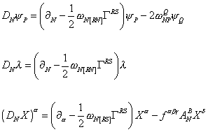
D_N [psi]_P = ([partial derivative]_N – ½w_N[RS] [capital gamma]^RS) [psi]_P – 2w_NP^Q [psi]_Q

D_N [lambda] = ([partial derivative]_N – ([partial derivative]_N – ½w_N[RS] [capital gamma]^RS)[lambda]

(D_NX)_[alpha] = ([partial derivative]_N – ½w_N[RS] [capital gamma]^RS)X^[alpha] -f^{[alpha][beta][delta]} A_N^BX^[delta]

The Yang-Mills strength is

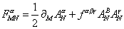
F_MN = ½[partial derivative]_M A_N^[alpha] + f^{[alpha][beta][delta]} A_M^BA_N^[gamma]

f^αβγ are the fine structure constants of the group

H_MNP = [partial derivative]_M B_NP – (G/[squareroot of 2]) ([omega]_MNP^YM – [omega]_MNP^L)

where G is the gravitational constant. The Yang-Mills Chern-Simons form is

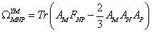
[omega]_MNP^YM = Tr(A_MF_NP – (3/2)A_MA_NA_P)

the Lorentz Chern-Simons form is

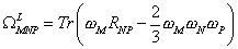
[omega]_MNP^L = Tr(w_M R_NP – (2/3) w_Mw_Nw_R)

and ψ_M is the gravitino, φ is the dilaton, λ is the dilatino, A_M^α is the gauge boson, X^α is the gaugino, and α is the E₈ x E₈ index. e_M^A is the zweibein, which is the two-dimensional version of the vielbein, referring to the two-dimensional world sheet. The geometry of a manifold is completely described in any coordinate patch by a set of orthogonal unit vectors called the vielbein, frame, or tetrad.

[e hat]_[alpha] = (e_[alpha])ⁱ [partial derivative]_i

where

[e hat]_[alpha] . [e hat]_[beta] = (e_[alpha])ⁱ (e_[beta])ⁱ g_ij = [eta]_{[alpha][beta]}

and where

[partial derivative]_i

is the coordinate basis vector, g_ij is the metric, and η_αβ is Minkowski spacetime. In any given number of dimensions, you take the German word for that number, and “bein”, which means “leg”, and that’s the name for the vielbein for that number of dimensions. Thus, a two-dimensional vielbein is called a zweibein. An n-dimensional vielbein is a set of n orthonormal basis vectors defined over the manifold. Vielbein is German for “many legs”, einbein is “one leg”, zweibein, is “two legs”, dreibein is “three legs”, vierbein is “four legs”, funfbein is “five legs”, elfbein is “eleven legs”, etc.

As I mentioned earlier, T-duality relates string theories by the following relation.

R_A R_B = l_s²

where A and B are the two string theories, R_A is the radius of the circle that one of the extra dimensions of A is compactified on, R_B is the radius of the circle that one of the extra dimensions of B is compactified on, and l_s is the string length, where l is lower case “L”. Let’s use dimensions where l_s = 1, so you have

R_A R_B = 1

R_A = 1/R_B

There are two types of excitations that a string can have. One is Kaluza-Klein excitations, which exist in any quantum field theory. The other is winding mode excitations which only exist for strings. It turns out that T-duality also relates these two types of excitations for two string theories.

In the context of string theory, Kaluza-Klein excitations exist because in order for the wave function e^ipx to be single valued, the momentum along the circle must be a multiple of 1/R.

p = n/R

where p is the momentum, R is the radius of the circle, and n is an integer. From the point of view of four-dimensional spacetime, this contributes

(n/R)²

to the square of the mass, which is the same as the square of the energy.

Winding mode excitations exist because a closed string can wind m times around the circular dimension. Imagine you are wrapping a rubber band around a pencil. This makes the following contribution to the energy.

E_m = 2[pi]RmT

If we are using units where the string length l_s = 1, then

T = 1/(2[pi])

so

E_m = mR

The combined energy squared of the Kaluza-Klein and winding mode excitations is

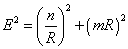
E² = (n/R)² + (mR)²

To this, you could also add the string oscillator contributions. If you have two string theories related by T-duality, and you exchange both m and n, as well as R and 1/R, it leaves the energy invariant.

m <-> n

R <-> 1/R

Together these two interchanges leave the energy invariant. This means that what is interpreted as a Kaluza-Klein excitation in one string theory is interpreted as a winding mode excitation in the T-dual theory, where the radius of the compactified dimension of the first theory is R, and of the second theory is 1/R.

One implication is that the usual geometric concepts break down at short distances, and classical geometry is replaced by quantum geometry, which is described mathematically by 2D conformal field theory. This also predicts a generalization of the Heisenberg Uncertainty Principle. According to this, Δx would be bounded below not just by 1/Δp but also by the string length, l_s. However, if you include non-perturbative effects, it might push this lower bound down to the Planck length.

Type IIA and IIB string theory are related by T-duality. The two heterotic string theories are also related by T-duality. In that case, one heterotic string has the SO(32) gauge group, and the other has E₈ x E₈. Therefore, you have to relate the two gauge groups. When the compactification on a circle is carried out, you have to include effects called Wilson lines. These break the gauge groups to SO(16) x SO(16) which is the common subgroup of SO(32) and E₈ x E₈.

To understand how superstring theory can produce the correct details of familiar traditional particle physics, you have to know about how the extra dimensions are compactified on a Calabi-Yau manifold. However, in order to just explain what a Calabi-Yau manifold actually is, I have to try to very briefly explain some advanced concepts in algebraic topology, which is a very complicated subject.

In 1943, Shiing-Shen Chern worked on characteristic classes and fiber bundles. In 1954, Eugenio Calabi conjectured the existence of a Kahler manifold with a Ricci-flat metric with a vanishing first Chern class, and a given complex structure and Kahler class. In 1976, Shing-Tung Yau proved the Calabi conjecture, and discovers Calabi-Yau space. In 1985, Candelas, Strominger, Horowitz, and Witten proposed using Calabi-Yau manifolds for the extra dimensions in heterotic string theory.

Projective geometry was essentially invented by Renaissance painters. Real projective space is RPⁿ. Points in RPⁿ are 1-dimensional subspaces of Rⁿ⁺¹, and are lines through the origin in Euclidean space. Complex projective space is CPⁿ. The Fubini-Study metric is the metric on complex projective space that has the maximal amount of symmetry.

A Calabi-Yau manifold can be generalized to any number of dimensions, but it’s usually described as having three complex dimensions. Since their complex structure may vary, you can think of them as having six real dimensions and a fixed smooth structure. A Calabi-Yau manifold has a non-vanishing harmonic spinor φ, which means that its canonical bundle is trivial.

The wedge product is the product of an exterior algebra, also called an alternating algebra or Grassmann algebra. If α and β are differential k-forms of degrees p and q respectively, then

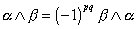
[alpha] /\ [beta] = (-1)^pq [beta] /\ [alpha]

It is not in general commutative but it is associative and bilinear.

Let’s say in R⁶, you have the coordinates x₁, x₂, x₃ , and y₁, y₂, y₃ so that

z_j = x_j + iy_j

gives it the structure of C³. Then

[phi]₂ = dz₁ /\ dz₂ /\ dz₃

is a local section of the canonical bundle. A unitary change of coordinates w = Az, where A is a unitary matrix, transforms φ by det A.

[phi]_w = det A [phi]_z

If the linear transformation A has determinant 1, meaning it is a special unitary transformation, then φ is defined as φ_z or φ_w. On a Calabi-Yau manifold, such a φ can be defined globally.

On a Riemannian manifold M, tangent vectors can be moved along a path by parallel transport. Think of the diagram in my paper on tensors. A closed loop at a base point p gives rise to an invertible linear map of TM_p, the tangent vectors at p. It is possible to compare closed loops by following one after another, and to invert them by going backwards. Therefore, a set of linear transformations arising from parallel transport along closed loops is a group called a holonomy group. Since parallel transport preserves the Riemannian metric, the holonomy group is contained in the orthogonal group O(n). If the manifold is orientable, then it is contained in the special orthogonal group. A generic Riemannian metric on an orientable manifold has a holonomy group of SO(n). Here are some Riemannian manifolds and their holonomy groups.

Kahler manifold (2n-dimensional) – U(n)

Calabi-Yau manifold (2n-dimensional) – SU(n)

hyper-Kahler manifold (4n-dimensional) – Sp(n)

quaternion Kahler manifold (4n-dimensional) – Sp(n) Sp(1)

Joyce manifold (7-dimensional) – G₂

One definition of a Calabi-Yau manifold, based on Riemannian geometry, is that it is a 2n-dimensional manifold whose holonomy group reduces to SU(n). Therefore, if n = 3, the Calabi-Yau manifold is a 6-dimensional manifold whose holonomy group reduces to SU(3).

Another definition of a Calabi-Yau manifold is that it is a calibrated manifold with a calibration form ψ which is algebraically the same as the real part of

dz₁ /\ dz₂ /\…/\ dz_n

Another definition of a Calabi-Yau manifold is that it is a Kahler manifold with vanishing Chern class. A Kahler manifold is a complex manifold for which the exterior derivative of the fundamental form Ω associated with a given Hermitian metric vanishes so dΩ = 0. In other words, it is a complex manifold with a Kahler structure. It has a Kahler form so it is also a sympletic manifold. It has a Kahler structure so it is a Riemannian manifold. A Kahler structure on a complex manifold combines a Riemannian metric of the underlying real manifold with a complex structure. A Kahler metric is defined such that near any point p, there exist holomorphic coordinates z_k = x_k + iy_k such that the metric has the form

g = [summation] dx_k x dx_k + dy_k x dy_k + O(| z |²)

A Chern class is a gadget defined for complex vector bundles. The Chern classes of a complex manifold are the Chern classes of its tangent bundle. The ith Chern class is an obstruction to the existence of (n – i + 1) complex linearly independent vector fields on that vector bundle. The ith Chern class is in the (2i)th cohomology group of the base space. For any collection of Chern classes such that their cup product has the same dimension as the manifold, this cup product can be evaluated on the manifold’s fundamental class. The resulting number is called the Chern number for that combination of Chern classes. Chern numbers are cobordism invariant. The fundamental class is the canonical generator of the nonvanishing homology group on a topological manifold. The cup product is a product on cohomology classes. Cobordism is where the union of two manifolds is the boundary of a compact (n + 1)-manifold. So to repeat, a Calabi-Yau manifold is a Kahler manifold with vanishing Chern class.

Calabi-Yau manifolds, as well as their moduli spaces, have many interesting properties, such as the symmetries in the numbers forming the Hodge diamond of a compact Calabi-Yau manifold. These symmetries, called mirror symmetries, also exist for another Calabi-Yau manifold which is a mirror of the first Calabi-Yau manifold. With mirror symmetry, two topologically distinct Calabi-Yau compactifications in string theory can give rise to identical models of particle physics. Calabi-Yau manifolds are also related to Kummer surfaces.

Let’s say you have a real manifold of dimension n. You can define the p-forms A^p, where p = 1, 2,…n, as

A^p = A_u1…updx^u₁ /\ dx^u₂ /\ …dx^u_p

where A is antisymmetric in its indices, and /\ is the wedge product which is also antisymmetric.

An exterior derivative of a p-form maps the p-form onto a (p + 1)-form by

dA^p = ([partial derivative]_{up + 1} A_u1…|up – [partial derivative]_u1 A_{up + 1…|ut}) dx^u₁ /\ dx^u /\ dx^u_p /\ dx^{u_{p + 1}}

A p-form is closed if dA^p = 0. A p-form is exact if A^p = dA^{p – 1}. Since d² = 0, an exact form is closed. If two closed forms differ by an exact form, they are in the same equivalence class. The collection of closed p-forms is called the cohomology group H^p. The number of different independent equivalence classes of p-forms is called the Betti number, b_p, and is the dimension of the cohomology group H^p.

The Betti numbers obey the Poincare duality.

b_p = b_{n – p}

where n is the dimension of the manifold. b₀ = 1 for any manifold for which b_n = 1. The Euler characteristic of a manifold is defined by

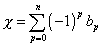
X = [summation over p from 0 to n] (-1)^p b_p

To study the homology group for a compact manifold of dimension n, you look at all its closed submanifolds. If

[partial derivative]B

is the boundary of a compact manifold B, then

[partial derivative]² = 0

since a boundary has no boundary. Therefore, the operation ∂ is analogous to the exterior derivative. A p-dimensional closed manifold may or may not be a boundary of a (p + 1)-dimensional closed manifold. If it is a boundary, ignore it. When two p-dimensional submanifolds M_p1 and M_p2 form the boundaries of a (p + 1)-dimensional manifold, they belong to the same equivalence class. Two points on a surface form the boundaries of a line, and therefore belong to the same equivalence class. The number of different equivalence classes gives the dimension of the homology group H_p, and gives the Betti number.

The Hodge decomposition theorem states that for a compact manifold, there is a one-to-one correspondence between a closed form and a harmonic form, which indicates the existence of a zero mode. This correspondence then enables you to obtain the number of massless modes from the Betti numbers.

Everything works the same for complex manifolds as with real manifolds with one difference. With real manifolds, there one index to each p-form. With complex manifolds, there are two indices to each form, called a (p, q)-form, where p is the holomorphic index, and q is the anti-holomorphic index.

A_p,q = A_{u1…up[v bar]1…[v bar]q} dz^u₁ /\ …dz_r^u /\ d[z bar]^{[v bar]₁}…/\ dz^{[v bar]_q}

Therefore, there are forms closed with respect to the holomorphic indices, anti-holomorphic indices, or both. The Betti numbers are b_{p, q}. The complex version of Poincare duality is

b_{p, q} = b_{n – p, n – q}

b_{p, q} is the number of massless modes.

The simplest example of a Kahler manifold is the space Cⁿ, which is n-tuples of the complex coordinates z₁, z₂… The Kahler potential φ is given by

[phi] = [summation over k] | z^k |²

This is not a compact manifold. To make it compact, you exclude the origin, and identify all points along lines passing through the origin. Let’s say

z^k ~ [lambda]z^k

for k = 1, 2…n, and you exclude the origin. The resulting manifold is called a CP^{n – 1} manifold. You have

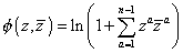
[phi](z, [z bar]) = ln (1 + [summation over a from 1 to n – 1] z^z [z bar]^a

This is not a Calabi-Yau manifold because the first Chern class of CP^{n – 1} is non-vanishing. Let’s look at submanifolds of CPⁿ which correspond to zero loci of homogenous polynomials.

Let’s say you have a CPⁿ manifold with homogenous polynomials p_i = 0 of degrees q. You then have

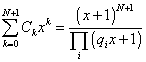
[summation over k from 0 to N + 1] C_k x^k = (((x + 1)^{N + 1})/([product series over i] (q_i x + 1))

where C_k are the Chern classes. The Calabi-Yau condition is C₁ = 0. This gives

N + 1 = [summation over i] q_i

As an example of a Calabi-Yau manifold, let’s look at a CP⁴ space. You have the following constraint

[summation over i from 1 to 5] z_i⁵ = 0

Calabi-Yau manifolds have SU(n) holonomy. Let’s say n = 3, so you have SU(3) holonomy. The Betti numbers b_{p, q} for the Calabi-Yau manifold are

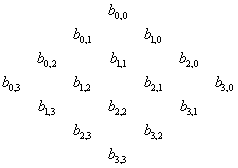
                      b_0,0

                b_0,1         b_1,0

        b_0,2         b_1,1          b_2,0

b_0,3         b_1,2         b_2,1          b_3,0

        b_1,3         b_2,2          b_3,1

                 b_2,3          b_3,2

                       b_3,3

This is called the Hodge diamond. From the Poincare duality, each Betti number on the top half is equal to one in the mirror image position in the bottom half. You have b_{0, 0} = b_{3, 3}, b_{0, 2} = b_{1, 3} , b_{0, 1} = b_{2, 3}, etc.

From this, you get

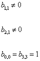
b_{1, 1} is not equal to 0

b_{2, 1} is not equal to 0

b_{0, 0} = b_{3, 3} = 0

The Euler characteristic of the manifold is given by

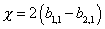
X = 2(b_{1, 1} – b_{2, 1})

For manifolds which are single CPⁿ, b_{1, 1} = 1. For products of CPⁿ, the manifold can be written as

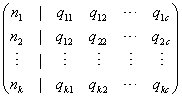
where q_ij is the power of the variable z_i in the jth polynomial. The total Chern class for the manifold

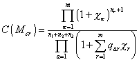
C(M_cr) = (([product series of pi from 1 to m] (1 + X_[pi])^{n_r + 1})/([product series of a from 1 to n₁ + n₂ + n₃] (1 + [summation over r from 1 to m] q_ar X_r)))

In order to compute b_{1, 1}, ignore the polynomials that mix the different CPⁿ‘s.

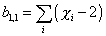
b_{1, 1} = [summation over i] (X_i – 2)

where χ_i is the Euler characteristic of the different submanifolds.

For a single CPⁿ manifold with several polynomial constraints

X = c₃ . [product series of i] q_i

where c₃ is the coefficient of x³.

Let’s look at a specific Calabi-Yau manifold. Let’s look at the one proposed by Tian and Yau. It is given by

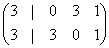
You have

b_{1, 1} = 2(X – 2)

where χ is the Euler characteristic of the manifold. You get

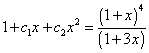
1 + c₁x + c₂x² = ((1 + x)⁴)/(1 + 3x))

From this, you get c₂ = 3, and χ = 9, so

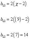
b_{1, 1} = 2(X – 2)

b_{1, 1} = 2(9 – 2)

b_{1, 1} = 2( 7 ) = 14

giving you b_{1, 1} = 14. The calculation of b_{2, 1} is done using deformation theory. It turns out that there is a one-to-one correspondence between the (2, 1)-forms and the independent polynomials by holomorphic transformations. These independent polynomials are independent complex structures of the manifold.

If you have the manifold proposed by Tian and Yau.

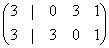
The total number of possible deformations is

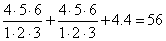
(4 x 5 x 6)/(1 x 2 x 3) + (4 x 5 x 6)/(1 x 2 x 3) + 4.4 = 56

Of these, 30 are related to the original polynomials by linear transformations, and three of the polynomials vanish. 56 – 30 – 3 = 23 Therefore, you have 23 independent complex structures, so b_{2, 1} = 23. So for this specific Calabi-Yau manifold, b _{1, 1} = 14, and b_{2, 1} = 23. Therefore, the Euler characteristic of this specific Calabi-Yau manifold is

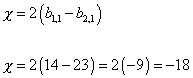
X = 2(b_{1, 1} – b_{2, 1})

X = 2(14 – 23) = 2(-9) = -18

Therefore, this Calabi-Yau manifold has a Euler characteristic of -18.

I have described the E₈ x E₈ heterotic superstring, and the Calabi-Yau manifold. Now, let’s take the E₈ x E₈ heterotic superstring theory, and compactify the extra dimensions on the correct Calabi-Yau manifold. The theory has N = 1 supersymmetry. Since this means you have N = 1 supergravity, you therefore have one massless graviton, from the e in the Lagrangian, and one massless gravitino, from the ψ_n. The φ gives rise to a massless dilaton. The λ gives rise to the dilatino. You also have the antisymmetric tensor B_μν. The action involving this field has a gauge invariance. After the gauge degrees of freedom are removed, you have one pseudo-scalar field a, which can be identified with the axion.

Let’s look at the gauge fields A_M^α, and their superpartners, the gaugino X^a in ten dimensions. Under E₈ x E₈, they transform as a

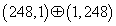
(248, 1) + (1, 248)

dimensional representation. Compactification that respects N = 1 supersymmetry requires that the gauge connection corresponding to the SU(3) subgroup be identified with the spin connection for the SU(3) part of the SO(6) group corresponding to the six compactified dimensions. Since the gauge field corresponding to the SU(3) subgroup has a non-zero vacuum expectation value, it breaks the gauge group E₈ x E₈ down to E₈ x E₆. Remember E₈ has the following maximal subgroups.

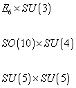
E₆ x SU(3)

SO(10) x SU(4)

SU(5) x SU(5)

The gauginos and gauge fields corresponding to the broken E₈ group have the following transformation properties under E₆ x SU(3)

{248} is a subset of (27, 3) + ([27 bar], [3 bar]) + (78, 1) + (1, 8)

Since the SU(3) gauge group is identified with the spin connection, the SU(3) gauge group indices become indices of the compactified manifold. Let’s divide the 10-dimensional spacetime index M into a spacetime coordinate u, and an internal coordinate m. The six m indices transform under SU(3) as

3 + [3 bar]

denoted by a and [a bar]. Then A_M^α contains A_{[α bar]}^α. Calabi-Yau manifolds with SU(3) holonomy have a covariantly constant antisymmetric tensor ε_abc. Multiplying by ε_abc, you can convert A_{[a bar]}^a into a (2, 1)-form

[epsilon]_abc A_{[a bar]}^a dz^b /\ dz^c /\ d[z bar]^{[a bar]}

Therefore, the (27, 3) part of the gauge field-gaugino system corresponds to closed (2, 1)-forms. Therefore, b_{2, 1} counts the number of {27}-dimensional superfields. Similarly, in the ([27 bar], [3 bar]) part of A_M^α, you can isolate part which transforms like A_{[a bar]}^{[b bar]} which can be converted into a (1, 1)-form

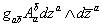
g_{a[b bar]} A_{[a bar]}^{[b bar]} dz^a /\ d[z bar]^{[a bar]}

Therefore, the number of massless {[27 bar]} superfields are given by the Betti-Hodge number b_{1, 1}. The number of generations of the particles is

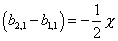
(b_{2, 1} – b_{1, 1}) = -½ X

There is a one-to-one correspondence between (2, 1)-forms and the polynomial deformations, so you have an explicit representation for the quark and lepton fields.

The starting gauge group for grand unification with Calabi-Yau type compactification is E₈ x E₆, with low energy matter fields transforming as {27}, of which the total number is given by b_{2, 1} of the corresponding manifold, and {[27 bar]}, given by b_{1, 1} of the manifold. The whole thing is then coupled to N = 1 supergravity. From this, you get the following gauge group breakdown scheme.

E₆ -> SO(10) x U(1)_X -> SU(5) x SU(1) x U(1)_X x U(1)_X’ -> SU(3) x SU(2) x U(1)_I3R x U(1)_{B – L} x U(1)_X

So the SU(3) group of the Calabi-Yau manifold breaks E₈ x E₈ to E₈ x E₆ . Then E₆ breaks to the SO(10) group, which is SO(10) x U(1)_X, which then breaks to the SU(5) group, which is SU(5) x SU(1) x U(1)_X x U(1)_X’, which then finally breaks to the Standard Model, which is SU(3) x SU(2) x U(1)_I3R x U(1)_{B – L} x U(1)_X.

In the following gauge group, you end up with the following particles.

(u d), [u bar], e⁺, [d bar], ([nu], e^–), [nu bar], g, (H₁⁺ H₁⁰), [g bar], (H₂⁰ H₂^_), n₀

where g is a g-quark, a new quark singlet, and n₀ is another singlet fermion. This is the particle content of the 27-dimensional representation of E₆. This is one generation. The number of fermion generations is given by

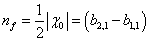
n_f = ½ | X₀ | = (b_{2, 1} – b_{1, 1})

The problem is the number of predicted generations is usually too big. If the Calabi-Yau manifold has a Euler number of -18, that would give ½ |-18| = 9 generations. We know from neutrino oscillations that there are only three generations. Therefore, you need a way to reduce to number of generations to three. Fortunately, you can reduce the Euler characteristic, χ₀, of the Calabi-Yau manifold by choosing an appropriate discrete symmetry group H that acts freely on the manifold R₀. It does not leave any point in the manifold fixed. The resulting manifold has the following Euler characteristic.

X = X₀/(dim H)

Let’s say you have a CP³ x CP³ manifold, and you have the following polynomials.

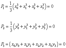
P₁ = 1/3 (x₀³ + x₁³ + x₂³ + x₃³) = 0

P₂ = 1/3 (y₀³ + y₁³ + y₂³ + y₃³) = 0

P₃ = (x₀y0 + x₁y₁ + x₂y₂ + x₃y₃) = 0

This Calabi-Yau manifold R₀ has a Euler number of χ = -18, and thus nine generations. To reduce the number of generations, consider the Z₃ group which acts freely on the manifold, and let it operate on the coordinates x_i and y_i where i = 0, 1, 2, 3

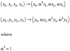
(x₀, x₁, x₂, x₃) -> (x₀, [alpha]² x₁, [alpha] x₂, [alpha] x₃)

(y₀, y₁, y₂, y₃) -> (y₀, [alpha] y₁, [alpha]² y₂, [alpha]² y₃)

where

[alpha]³ = 1

This reduces χ to -6

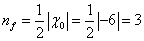
n_f = ½ | X₀| = ½ | -6 | = 3

so you have three generations of fermions. Therefore, if you compactify the extra dimensions on this specific Calabi-Yau manifold, you end up with three generations of quarks and leptons recognizable as the familiar particles from the Standard Model.

The discrete symmetry group H can also be used to break the gauge groups through symmetry breaking, which is good because otherwise the proton would have a lifetime of only 10^-15 seconds. A function ψ acting on R is equivalent to a function on R₀ if

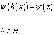
[psi] (h (x)) = [psi](x)

h is a member of H

Since the Lagrangian is E₆-invariant, the following weaker condition is sufficient.

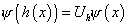
[psi] (h (x)) = U_h [psi](x)

where U_h is an element of the E₆-group which provides a homomorphism of H into the group H₆. Since under a gauge rotation

[psi] -> V[psi]

you have

[V, U_h] = 0

The surviving group below the compactification scale is the one that commutes with the embedding of H in E₆, and is therefore a smaller group.

In the process of compactification, all E₆-gauge field strengths in ten dimensions must vanish. In a simply connected manifold, F_mn = 0 nears that of A_m = 0 up to the gauge transformations. However, for a multiply connected manifold, this is not true since

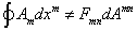
[path integral] A_m dx^m is not equal to F_mn dA^mn

Since A_m transforms as the adjoint representation of E₆

A_m is not 0

reduces the gauge group without reducing its rank.

To use this for E₆, you need functions of A_m which are unitary operators such as

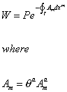
W = Pe^{(-[path integral around gamma]A_mdxm)} where

A_m = [theta]^a A_m^a

and where a is the E₆ index, and γ is a closed loop in the multiply connected space. W is called the Wilson loop integral. When

A_m^a is not 0

you have

W is not 0

and it leads to a breakdown of the E₆ symmetry.

For a Z_n group, which is abelian, Wⁿ = 1, and you can parametrize W as

W = e^{2[pi]i[summation over a from 1 to b] [lambda]_a[theta]_a}

where θ_a are elements of the Cartan subalgebra of the E₆ group, λ_a are real parameters, and a = 1, 2,…6.

The mass of a gauge boson, whose weight factor is given by α is proportional to α. λ, where α is a six-component vector for the E₆ group. When

[alpha] . [lambda] = 0

you get an unbroken symmetry group. Using the root vectors of E₆, in order to keep SU(3) x SU(2) x U(1) unbroken, λ must have the following form

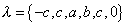
[lambda] = {-c, c, a, b, c, 0}

where a, b, and c are arbitrary constants. If they are totally arbitrary, the unbroken group is the Standard Model group SU(3) x SU(2) x U(1). If they are not totally arbitrary, the group that is unbroken is larger than the Standard Model group.

Here we have assumed that only abelian groups break E₆. However, you can also consider non-abelian groups. An advantage of using non-abelian groups is that the breaking at the Planck scale also reduces the rank of the group so you could avoid the problem of rapid proton decay.

In order for the E₆ type superstring models to be phenomenologically viable, you need at least one intermediate scale, and possibly two. There are three main points that have to be satisfied. First of all, baryon number violating processes must be suppressed to an acceptable level. Second of all, the evolution of coupling constants depends on the β-function for the gauge theory. As I said in the section on supersymmetry, the existence of extra fermions slows down the evolution of the coupling constants. In the E₆ supergravity model, there is an extra quark called the g-quark. This causes the SU(2) coupling to grow beyond the electroweak scale while the QCD coupling is fixed beyond the electroweak scale. This could destroy the unification of the coupling constants. Third of all, the E₆ group is left-right symmetric. Left-right symmetric models contain a right-handed neutrino that allows you to give masses to the neutrinos. However, all by itself, the mass of the neutrinos would be too large. You have to explain the great discrepancy between the masses of the neutrinos and the other leptons. The usual solution is the see-saw mechanism. However, in superstring theory, you can’t use the normal see-saw mechanism. The solution to the first two problems is at least one intermediate scale. The solution to the third problem is to have a generalized see-saw mechanism.

Let’s say you have the following compactification.

W = [lambda]₁ Q Q^c [phi] + [lambda]₂ LL^c [phi] + [lambda]₃ (QQg + Q^c Q g^c) + [lambda]₄ (QLg^c + Q^c L^c g) + [lambda]₅ Tr [phi]² n₀ + [lambda]₆ gg^c n₀

where

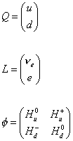
Q = (u, d)

L = ([nu], e)

Let’s look at the baryon number interactions, which are the couplings λ₃ and λ₄. The g-quark acquires a mass of

n₀is not 0

The effective QQQL-type Hamiltonian is given by

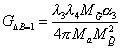
G_{[delta]B = 1} = ([lambda]₃ [lambda]₄ M_{[G tilda]} [alpha]₃)/(4[pi]M_a M_{[Q tilda]}²)

Let’s say

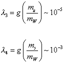
[lambda]₃ = g(m_u/m_W) ~ 10^-5

[lambda]₄ = g(m_s/m_W) ~ 10^-3

Then

G_{[delta]B = 1} = 10^-16/m_g

Therefore

m_g > 10¹⁴ GeV

Therefore you must have

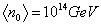
n₀ = 10¹⁴ GeV

for baryon number violation to be consistent with experiment. Therefore, you need at least one intermediate scale. This would also solve the problem of the evolution of the coupling constants since the g-quark would start contributing to the evolution of the coupling constants only above 10¹⁴ GeV.

The problem of explaining the small neutrino masses is normally done by the see-saw mechanism which requires generating large Majorana masses, which requires a Higgs boson with a B – L quantum number 2. There is no such particle in string theory. Therefore, you can’t use the normal see-saw mechanism. However, you can instead use a generalized see-saw mechanism by adjoining a 2-component chiral neutral lepton S to each pair of neutrino and anti-neutrino. You can then write the following 3 x 3 matrix.

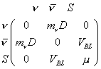
In order to generate the [ν bar]S entry, you need a Higgs boson with SU(2)_R x U(1)_{B – L} quantum number (½, 1), which is part of the {27}-dimensional representation of E₆.

If V_BL has a value of 1 TeV, for u = 10 – 100 GeV, then m_ν is acceptably small. S could be the B – L gaugino or any other E₆ singlet. Therefore, by including an intermediate breaking scale, and a modified see-saw mechanism, you can solve the problems of baryon number violation, unification of the coupling constants, and smallness of neutrino masses. Therefore, there are no obvious phenomenological problems with E₈ x E₈ superstring theory compactified on a CP³ x CP³ Calabi-Yau manifold.

Therefore, if you take E₈x E₈ heterotic superstring theory, and compactify six of the ten dimensions on a specific Calabi-Yau manifold, CP³ x CP³, you get a theory that includes N = 1 supergravity, and thus the spin-2 graviton, Yang-Mills fields, and thus the spin-1 gauge bosons, and then through the 27-dimensional representation of E₆, all the quarks and leptons of the Standard Model, in three generations, and also with a method of breaking the symmetry of the gauge groups through an intermediate scale that preserves the long proton lifetime. That is an amazingly impressive achievement.

At the same time, I don’t want to overstate the success of superstring theory. It wasn’t until 2002 that we could calculate scattering amplitudes at the two loop level. In 1982, Michael Green and John Schwarz were able to calculate scattering amplitudes of Type II strings at tree level and first loop. In 1986, Gross, Harvey, Martinec, and Rohm were able to calculate scattering amplitudes of the Heterotic string at tree level and first loop. In 2002, Eric D’Hoker and D. H. Phong were able to calculate scattering amplitudes of Type II and Heterotic strings up to second loop. The reason it took so long to go from one loop to two loops is that in the RNS formalism, there is the emergence from the gauge fixing procedure of odd Grassmann-valued supermoduli. They eventually solved this problem using a superspace formulation of the worldsheet. They gave a construction from first principles for an unambiguous and slice-independent two-loop superstring measure on moduli space for even spin structure.

In superstring theory, the extra dimensions are usually compactified on a Calabi-Yau manifold, although people have successfully compactified the extra dimensions on other manifolds, such as K₃ or K3, which is a manifold with SU(2) holonomy, and even other types of topology, such as orbifolds. An orbifold is a slight generalization of a manifold that allows singularities. For instance, you could think of the rotation group G of a given polyhedron, which is a subgroup of the rotation group SO(3). Let’s say you have R³, and define two points (x, y, z) and (x’, y’, z’) to be equal if you can get from one to the other by a rotation in G. The resulting space is not a manifold. For instance, it has a singularity at the origin. However, it is an orbifold. In this example, it’s called “R³ modulo the action of G”.

Landau-Ginzburg models were originally used to describe phase transitions. A supersymmetric generalization of Landau-Ginzburg models has been studied in the context of superstring compactification. The expectation value of an n-tuple of fields is controlled by a potential, which in supersymmetric models, is the square of the magnitude of the gradient of a holomorphic function. This gives rise to an orbifold that extra dimensions can be compactified on. There are many Landau-Ginzburg orbifolds that give rise to identical physics as specific Calabi-Yau manifolds.

There are two basic ways of formulating superstring theory. You can put the supersymmetry on the two-dimensional string world sheet, which is called the Ramond-Neveu-Schwarz formalism, or the RNS formalism. You can also put the supersymmetry on the ten-dimensional spacetime that the strings are moving through, which is called the Green-Schwarz formalism, or the GS formalism. What we’ve been discussing so far has been the RNS formalism, which is much easier, and therefore more common, although it obscures the fact that the theory is truly supersymmetric in the traditional sense. The GS formalism is considerably more difficult technically, although the physics is perhaps more transparent.

The RNS formalism is easier because you are working in two dimensions, meaning the two dimensions of the world sheet. This world sheet supersymmetry also requires spacetime supersymmetry, which is what we’re interested in, although the proof is long and difficult, and the supersymmetry is not manifest at the level of the action.

In the Green-Schwarz formalism, you are dealing directly with spacetime supersymmetry. In superstring theory, you have 10 dimensions, meaning eight degrees of freedom, which are eight transverse coordinates in the light cone gauge. The other two degrees of freedom can be eliminated by a gauge transformation. Therefore, you have eight bosonic degrees of freedom, and you need to get eight fermionic degrees of freedom in order to have the same number of bosonic and fermionic degrees of freedom. However, a spinor in 10 dimensions has 32 complex components. If you impose Majorana and Weyl conditions, you can reduce this to 16. The resulting representation of the Lorentz group is irreducible. How do you then reduce the number of fermionic degrees of freedom from 16 to 8?

Fortunately, there exists a type of symmetry called kappa symmetry, or κ-symmetry, originally proposed by Seigel, under which half of the fermionic degrees of freedom can be gauged away. In 1981, Michael Green and John Schwarz found an action with kappa symmetry, that they used to gauge away half of the fermionic degrees of freedom, reducing the number of fermionic degrees of freedom from 16 to 8, so you ended up with the same number of bosonic and fermionic degrees of freedom. You end up with an action with manifest supersymmetry.

This is the advantage over the RNS formalism. However, the RNS and GS formalisms are equivalent to each other. Most string theorists work in the RNS formalism because gauge fixing the kappa symmetry is extremely difficult. If you want to preserve manifest Lorentz invariance, you end up with an infinite number of ghosts.

Let’s discuss the GS formalism of superstrings in more detail. Let’s start with the N = 1 and N = 2 superspaces which are identified with the supertranslation groups. The supertranslation algebras are spanned by the 10-momentum P_u, and one or more Lorentz spinor charges. The minimal spinor in d = 10 is Majorana and chiral. A Majorana spinor Q is one for which

[Q bar] = Q^T C

where the bar represents the Dirac conjugate, and C is the antisymmetric real charge conjugation matrix. There exists a representation of the Dirac algebra called the Majorana representation in which the Dirac matrices are real. In this representation

C = [capital gamma]⁰

and a Majorana spinor is a real 32-component spinor. A chiral spinor Q is one for which

[capital gamma]₁₁ Q_± = ± Q

where Γ₁₁ is the product of all ten Dirac matrices. It satisfies

([capital gamma]₁₁)² = 1

and is therefore real in the Majorana representation. A chiral Majorana spinor has 16 independent real components.

The N = 1 supertranslation algebra is

{Q_[alpha]⁺, Q_[beta]⁺} = (C[capital gamma]^u P⁺)_{[alpha][beta]}P_u

where Q⁺ is a chiral Majorana spinor, P_u is the 10-momentum, and P⁺ projects onto the positive chirality subspace. The choice of positive or negative chirality is a convention. An element of the supertranslation group is obtained by exponentiation of the algebra element

X^u P_u + [theta bar]₊ Q⁺

where X^u are d = 10 spacetime coordinates, and θ₊ is an anti-chiral and anticommutating Majorana spinor coordinate. There are two N = 2 supertranslation algebras, according to whether the two supersymmetry charges have the same or opposite chirality. If they have opposite chirality, you can assemble them into a single non-chiral Majorana charge Q. This leads to the IIA algebra.

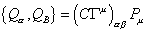
{Q_[alpha], Q_[beta} = (C[capital gamma]^u)_{[alpha][beta]} P_u

If the two supersymmetry charges have the same chirality, you can assemble them into the SO(2) doublet Q^+I, where I = 1, 2. You then get the IIB algebra.

{Q_[alpha]^+I, Q_[beta]^+J} = [delta]^IJ (C[capital gamma]^u P⁺)_{[alpha][beta]} P_u

With these supertranslation algebras, you can then construct superstring world sheet actions in the Lorentz covariant Green-Schwarz formulation, where the fields are maps from the world sheet to the superspace. You need the following supertranslation invariant superspace 1-forms on the three possible superspaces.

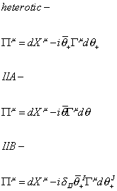
heterotic-

[capital pi]^u = dx^u – i[theta bar]₊ [capital gamma]^u d[theta]₊

IIA-

[capital pi]^u = dx^u – i[theta bar] [capital gamma]^u d[theta]

IIB-

[capital pi]^u = dx^u – i[delta]_JJ [theta bar]₊^I [capital gamma]^u d[theta]₊^J

The first is heterotic. The second is IIA. The third is IIB. The N = 1 superspace case is relevant to the heterotic strings. The Type I superstring is derived from the IIB superstring. The world sheet coordinates are

[xi]ⁱ = ([tau], [sigma])

and

[capital pi]_i^u

is the 10-vector components of the induced world sheet 1-forms. In the heterotic case, you have

[capital pi]_i^u = [partial derivative]_iX^u – i[theta bar]₊ [capital gamma]^u [partial derivative]_i [theta]₊

where

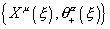
{X^u([xi]), [theta]₊^[alpha] ([xi])}

are the world sheet fields.

If you set the string tension to one, you can then write the Nambu-Goto action

S_NG = -[integral] d² [xi] [squareroot of (-det ([capital pi]_i . [capital pi]_j)]

This is not the complete action because you also need a Wess-Zumino term. To construct it, you need super-Poincare closed forms in superspace. You need the following 3-forms

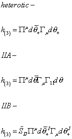
heterotic-

h₍₃₎ = [capital pi]^u d[theta bar]₊ [capital gamma]_u d[theta]₊

IIA-

h₍₃₎ = [capital pi]^u d[theta bar] [capital gamma]_u [capital gamma]₁₁ d[theta]

IIB-

h₍₃₎ = [S tilda]_JJ [capital pi]^u d[theta bar]₊^I [capital gamma] d[theta]₊^J

where Γ₁₁ is the product of the ten Dirac matrices Γ^u, and [S tilda]_JJ are the entries in the following 2 x 2 matrix.

In the above 3-forms, the first is for the heterotic. The second is for IIA. The third is for IIB. Next, you need the heterotic 7-form.

h₍₇₎ = [capital pi]^u₁…[capital pi]^u₇ d[theta bar]₊ [capital gamma]_u1…u7 d[theta]₊

These forms are closed due to Dirac matrix identities valid in d = 10 so locally you can write h = db.

Given a (p + 2)-form h_{(p + 2)}, you can write to a super-Poincare invariant Wess-Zumino type action for a p-dimensional object, or p-brane, by integrating the (p + 1)-form b_{(p + 1)} over the (p + 1)-dimensional world volume. Thus h₍₇₎ = db₍₆₎ is relevant to 1-branes, meaning strings. You can now write down the Wess-Zumino term in the GS superstring action

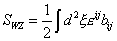
S_WZ = ½ [integral] d² [xi] [epsilon]^ij b_ij

The combined action is the sum of the Nambu-Goto and Wess-Zumino actions.

S = S_NG + S_WZ

The combined action has a fermionic gauge invariance called kappa symmetry or κ-symmetry, which allows half of the components of θ to be gauged away. When you choose a physical gauge, half of the original spacetime symmetries are linearly realized world sheet supersymmetries. Without κ-symmetry, they would be non-linearly realized. Thus, κ-symmetry is essential for equivalence with the world sheet supersymmetric RNS formalism of superstring theory.

The type II superstrings are closed strings whose covariant GS action is just S = S_NG + S_WZ, and for which the world sheet fields are all periodic. The fermions are actually world sheet scalars in this formalism. They become world sheet spinors only after gauge-fixing the κ-symmetry. The heterotic strings are closed strings based on the action S = S_NG + S_WZ for N = 1 superspace, but because of conformal invariance of the first quantized string, you also need a heterotic action involving 32 world sheet chiral fermions.

[zeta]^A A = 1, 2,…32

If you choose these to transform as half-densities, then the heterotic action is

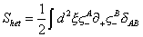
S_het = ½ [integral] d² [xi] [zeta]^A [partial derivative]₊ [zeta]_–^B [delta]_AB

where ∂₊ is a chiral world sheet derivative. Therefore, the GS action for the heterotic string is

S = S_NG + S_WZ + S_het

The world sheet fermions ζ^A could be periodic or anti-periodic, so there seem to be many possible sectors in the full Hilbert space of the first quantized string. However, quantum consistency reduces the choices to the SO(32) and E₈ x E₈ heterotic strings.

There are many times when you are teaching somebody something, and you say something that is technically inaccurate, but is sufficiently accurate for the purpose, and then when the student reaches a more advanced level, they learn a more accurate version. In elementary school, the orbits of the planets are described as circular. In high school, they are described as ellipses. In college, a student might learn that they are actually egg-shaped, with the pointy end pointing to the Sun. A professional planetary astronomer calculating the positions of the planets with extreme precision would have to take into account the gravitational attraction of all the other planets and smaller bodies in the solar system. This is not to say you are lying to the elementary or high school students. What you tell them is sufficiently accurate for the purpose. Another example is in my paper on the Standard Model when I said that QCD predicts quark confinement, meaning quarks are permanently bound inside hadrons, or least have been since shortly after the Big Bang. However, according to some recent theories, you could have quarks outside of hadrons today, in certain neutron stars called quark stars, or even briefly in particle accelerators. However, you should not tell that to someone who is trying to learn QCD since the whole idea of QCD is to explain quark confinement. You don’t want to confuse someone who is just beginning to learn it.

We have reached a point where I should probably mention that the names of the gauge groups that are commonly used by particle physicists are not actually technically accurate. Particle physicists use the names all the time but a mathematician would complain that the commonly used names are not the names of the actual groups involved. Mathematicians usually demand a higher level of technical accuracy in the nomenclature then physicists. A Lie algebra is a logarithm of a Lie group, and a Lie group is an exponential of a Lie algebra. There are several different Lie groups that have the same Lie algebra. What we have been calling the Standard Model gauge group SU(3) x SU(2) x U(1) is more accurately described as

[SU(3) x SU(2) x U(1)]/Z₆

All of the SU(n) groups we have mentioned are actually SU(n)/Z₆. For instance, SU(5) is really SU(5)/Z₆. What we have been calling SO(10) is actually Spin(10). The E₈ x E₈ group is actually the semi-direct product

(E₈ x E₈) [triangle] Z₂

where Z₂ acts by exchanging the E₈ factors. The SO(32) group of Type I and Heterotic SO(32) superstring theory is actually

Spin(32)/Z₂

also called Semispin(32). However, there is something different about this last example, which is that there is a downside to confusing the group you call it with the group it really is. With all the other examples, it does not make any difference. One group is called the cover for the other. That means you can use the technically inaccurate names with no negative repercussions.

For instance, SO(10) grand unification uses a certain 16-dimensional multiplet that does not correspond to any representation of SO(10). It is actually a representation of Spin(10). However, you can just use the name SO(10) to mean Spin(10). There is no harm done. Every representation of SO(10) is automatically a representation of Spin(10), because Spin(10) is a cover for SO(10). Similarly, you can write SU(3) x SU(2) x U(1) for [SU(3) x SU(2) x U(1)]/Z₆ since every representation of the latter is a representation of the former. However, you can not do that with SO(32) and Spin(32)/Z₂ because neither is a cover for the other. Both have representations which can’t be regarded as representations of the other.

The T-duality of the two heterotic string theories relies on relating E₈ x E₈ and SO(32) through their supposed common subgroup SO(16) x SO(16). However, no such common subgroup exists. Not only that, but neither of the actual representative subgroups covers the other. Furthermore, each has representations which are not representations of the other, but which are crucial in establishing T-duality. Also, you have Wilson loops which behave in a way that depends very delicately on the various subgroups of Spin(32)/Z₂ and Spin(16)/Z₂. The local simplicity of the duality arguments conceals considerable complexity at the global level. Therefore, in the case of the so-called SO(32) group of superstring theory, there is good reason to remember that the actual group is Spin(32)/Z₂, also called Semispin(32). That said, unless you are dealing with the finer points I mentioned above, most string theorists usually just go ahead and call it SO(32), while keeping in mind that really it’s not.

The five superstring theories are related to each other by the T, S, and U dualities. This turned out to be a clue of the next great advance in superstring theory that took place during the second superstring revolution, starting in 1994. It turned out that the five superstring theories are all just different manifestations of one single underlying theory. This is a good thing since we would rather have one instead of five fundamental theories of the Universe. Also, this opened the door to discussing string theory non-perturbatively, and it was assumed that the perturbative expansion is not the whole story, and you would have to take non-perturbative effects into account in order to get an accurate view of the Universe. In string theory, the coupling constant, g_s, is determined by the expectation value of a scalar field called the dilaton. There is no reason to assume it’s small, which you have to do in order to assume that the perturbative expansion is an accurate approximation. The five string theories turn out not to be distinct theories. Instead, each of the five theories represents a perturbative expansion of a single underlying theory about a distinct point in the moduli space of the quantum vacua. Interestingly, there is also a sixth point in the moduli space that corresponds to an 11-dimensional supergravity theory. Unfortunately, both the 11-dimensional supergravity theory and the underlying theory are called M-theory. This is unfortunate terminology since you should not confuse them. The 11-dimensional supergravity theory is not any more fundamental than the five string theories. Some authors have thought up various different names to call them, in an attempt to distinguish them, and avoid confusion, but so far, there is no consensus. Usually, it’s obvious from the context. I will usually refer to the fundamental underlying theory as M-theory, and call the other one 11d supergravity. You might also wonder, what does the “M” stand for? In fact, nobody knows. Different people claim that the “M” stands for magic, mystery, meta, matrix, membrane, murky, or mother of all theories.

However, this lack of understanding or consensus about what the “M” stands for, or what the word “M-theory” refers to, is perhaps appropriate. M-theory is literally the most advanced theory in all of physics. This is our current view of the Universe. You can look at the history of particle physics starting with the ancient Greeks, and go all the way up to M-theory, which is the most advanced theory that humanity has yet achieved. M-theory is the most advanced theory we currently possess. However, one aspect of that fact is that it is such a recent development, we haven’t figured out what exactly it is yet. Therefore, when studying M-theory, you are witnessing physics in progress, as we are in the process of figuring out what exactly it is.

The five string theories are well understood as perturbation expansions. They have consistent perturbation expansions of on-shell scattering amplitudes. The type II and the heterotic string theories have only closed strings so they have particularly simple perturbation expansions. There is a unique Feynman diagram at each order of the loop expansion. The Feynman diagrams are world sheets. A given L-loop diagram is a closed orientable genus-L Riemann surface. Incoming and outgoing particles are represented by N punctures on the surface.

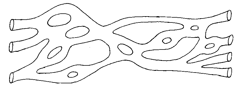
A given diagram represents a well-defined integral of dimension 6L-2N-6, where L is the genus of the world sheet, and N is the number of punctures, meaning the number of incoming and outgoing particles. The integral contains no divergences, despite containing the spin-2 graviton. String and supersymmetry contributions are responsible for amazing cancellations. Type I superstring theory contains both open and closed strings, so the perturbation expansion is more complicated. Various world sheet Feynman diagrams at a given order have to be combined to cancel divergences and anomalies.

T-duality can be understood perturbatively. This duality is between two string theories where one spatial dimension is compactified on a circle. It also holds true for more complex manifolds, such as Calabi-Yau manifolds, but obviously it’s easiest talk about in the context of a simple manifold with one dimension compactified on a circle. Let’s say you have two superstring theories A and B, each on a R⁹ x S¹ manifold. If the radius of the circles that the extra dimensions are compactified on are R_A and R_B, then you have

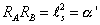
R_A R_B = l_s² = [alpha]’

where l_s is the string length, and α’ is the universal Regge slope, which is the string length squared. T-duality means that shrinking the circle to zero in one theory corresponds to expanding the circle in the other theory. Type IIA and Type IIB superstring theories are T-dual. This means that if you take the non-chiral Type IIA superstring theory, and compactify one dimension on a circle of radius R, and let R go to zero, it turns into the Type IIB theory in ten dimensions.

Instead of thinking of them as two theories that are related, you could instead think of them as only one theory. What we call two theories are just two points on a continuous spectrum. The radius R is actually the vacuum value of a scalar field, which arises as an internal component of the 10d metric tensor. Therefore, the Type IIA and Type IIB superstring theories are just two limiting points on a continuous moduli space of quantum vacua. The two heterotic superstring theories are also T-dual, although in that case, it’s more complicated because of the different gauge groups. If you apply T-duality to Type I superstring theory, it turns into an unusual variation of itself called Type IA or Type I’.

In the 1970’s, many people were working on point particle theories of supergravity, totally independent of string theory. In these theories, making supersymmetry a local symmetry naturally led to a spin-2 particle that could be identified with the graviton. However, these theories were non-renormalizable, as were all pre-string attempts to quantize gravity. In 1978, Cremmer, Julia, and Sherk developed a specific supergravity theory that existed in 11 dimensions. It had 32 conserved charges, and three kinds of fields. The first is the graviton field with 44 polarizations. The second is the gravitino field with 128 polarizations. The third is a three index gauge field, C_μνρ, with 84 polarizations. The supergraviton is a quantum mechanical mixture of these fields. Of course, 11d supergravity is non-renormalizable. 11-dimensional supergravity does not have a perturbation expansion. Also, it did not seem to have a mechanism for generating chiral fermions. Therefore, it did not seem promising that it would be an important theory.

However, early on, some people noticed a possible connection between the 11d supergravity and Type IIA superstring theory. The IIA supergravity and the 11d supergravity were similar. The main difference was that 11d supergravity was 11-dimensional, and the Type IIA supergravity was 10-dimensional. There was some sort of subtle connection between these two very different theories that remained a curiosity for many years. In 1987, Bergshoeff, Sezgin, and Townsend tried to rework the 11d supergravity theory as a theory of two-dimensional membranes analogous to superstring theory which was a theory of one-dimensional strings. The field equations of 11d supergravity admit a solution that describes a supermembrane. The energy density is concentrated in a two-dimensional surface. A 3d world volume description of the dynamics of this supermembrane is analogous to the 2d world volume actions of superstrings. They couldn’t really get this theory of supermembranes to work, but it further pointed to a connection between the 11d supergravity and superstrings. Then it was realized that if you take this theory, and just reduce the dimension of the supermembrane world volume, you get the previously known Type IIA superstring world volume. This seemed to strongly suggest something profound, but no one could figure out what exactly it was, and again it remained a tantalizing puzzling curiosity. Then in 1995, P. K. Townsend and Edward Witten made a major breakthrough. In a shocking discovery, they determined that the Type IIA superstring theory really is 11-dimensional. Everyone had always thought it was 10-dimensional, but the whole time, it was actually 11-dimensional. It turned out that Type IIA superstring theory actually has an 11th dimension compactified on a circle, in addition to the previously known 10 dimensions. The reason why nobody had noticed this before is because it was a non-perturbative effect, and the theory had only been studied perturbatively.

The 11-dimensional supergravity, and thus M-theory, has no dimensionless parameters. The only parameter is the 11-dimensional Newton constant, which raised to the power of -1/9 gives the 11-dimensional Planck mass, m_p. When M-theory is compactified on a circle, the spacetime geometry is R¹⁰ x S¹, so you have another parameter, which is the radius of the circle. The parameters of Type IIA superstring theory are the string mass scale, m_s, and the dimensionless string coupling constant, g_s. Therefore, you can identify compactified M-theory with Type IIA superstring theory by

m_s² = 2[pi]Rm_p

g_s = 2[pi]Rm_s

where m_p is the Planck mass, m_s is the string mass scale, g_s is the string coupling constant, and R is the radius of the circle that the 11th dimension is compactified on. You then have

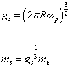
g_s = (2[pi]Rm_p)^3/2

m_s = g_s^1/3 m_p

Therefore, the Planck length is shorter than the string length scale at weak coupling by a factor of (g_s)^1/3.

In traditional superstring theory, you have a perturbation expansion in powers of g_s at fixed m_s. This is equivalent to an expansion about R = 0. The strong coupling limit of Type IIA superstring theory corresponds to decompactification of the 11th dimension. If you have Type IIA superstring theory, and take the coupling constant g_s to infinity, you end up with M-theory. Therefore, M-theory is Type IIA superstring theory at infinite coupling. You see how the 11th dimension would not be detected in string perturbation theory, which is at low coupling.

M-theory is a theory of membranes which are two-dimensional surfaces. It turns out that if you take an M2-brane of M-theory, and wrap one of its dimensions around the compact circular dimension, it looks the same as a superstring in Type IIA theory. Therefore, Type IIA superstrings actually are M-theory M2-branes with one of their dimensions wrapped around the 11th dimension which is compactified on a circle. If the string tension, T_F1, is the energy per unit length, and the membrane tension, T_M2, is the energy per unit volume, they are related by

T_F1 = 2[pi]RT_M2

Also, you have

T_F1 = 2[pi]m_s²

T_M2 = 2[pi]m_p²

From this, you get

m_s² = 2[pi]Rm_p³

At high coupling, Type IIA theory becomes 11-dimensional, where the 11th dimension is compactified on a circle. At low coupling, the radius of the circle is too small for it to be noticed. This is similar to the analogy I gave earlier with the garden hose. The E₈ x E₈ heterotic superstring theory also becomes 11-dimensional. In that case, the extra dimension is a line segment between the two 10-dimensional boundaries. Imagine you had two parallel planes separated by a line segment. If the line segment was very small, it would look like a plane. As the line segment got longer, you notice it was a three-dimensional space bounded by two planes. Here you have two 10-dimensional spaces separated by a line segment. At the low coupling, the line segment is short, and you think it’s 10-dimensional space. At high coupling, the line segment gets longer, and you realize it’s 11-dimensional space bounded by two 10-dimensional spaces. In E₈ x E₈ superstring theory, you have one E₈ current algebra on each of the two 10-dimensional string boundaries. The string coupling is

g_s = L^3/2

where L is the length of the line segment.

Even though people talk about these theories becoming 11-dimensional, they are really always 11-dimensional. You just don’t notice the 11th dimension at weak coupling, meaning perturbatively. We know that the Type IIA superstring theory and the 11-dimensional supergravity are really the same theory. We know Type IIA superstring theory and E₈ x E₈ Heterotic superstring theory are really 11-dimensional. We know from T-duality, that the two Type II superstring theories are really the same theory, and the two heterotic string theories are really the same theory. We know from S-duality, that the Type I superstring theory and the SO(32) Heterotic superstring theory are really the same theory. Therefore, we know that all the five superstring theories, and also the 11-dimensional supergravity theory, are all really the same theory, and that one theory is 11-dimensional.

Since M-theory is a theory of membranes, this then ties in with D-branes, which I described earlier as a recent feature of superstring theory. If you want to specify the dimension of a D-brane, you call it a Dp-brane, where p is the dimension. The world volume swept out by a Dp-brane has p + 1 dimensions. The tension of a D-brane is given by

T_D = (2[pi]m_s^{p + 1})/g_s

Notice that the tension depends on the coupling constant. The D-branes carry a charge that couples to a gauge field in the RR sector of the theory. p takes even values in IIA theory, and odd values in IIB theory.

The D2-brane of Type IIA superstring theory corresponds to the supermembrane of M-theory with one of its dimensions compactified on a circle. The tension is

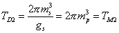
T_D2 = (2[pi]m_s³)/g_s = 2[pi]m_p³ = T_M2

where T_D2 is the tension of the D2-brane, T_M2 is the tension of the M2-brane, m_s is the string mass scale, m_p is the Planck mass, and g_s is the string coupling constant. The mass of the first Kaluza-Klein excitation of the 11d supergraviton is 1/R, which can be identified with the D0-brane. Every p-brane has a magnetic dual. The magnetic dual of a p-brane in d dimensions is a (d – p – 4)-brane. So for a D2-brane, which is the membrane in M-theory, you have

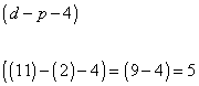
(d – p – 4)

( (11) – (2) – 4) = 9 – 4 = 5

This is called an M5-brane. It’s tension is

T_M5 = 2[pi]m_p⁶

If you wrap one of its dimensions around a circle, you get a D4-brane with tension

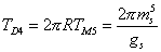
T_D4 = 2[pi]RT_M5 = (2[pi]m_s⁵)/g₅

where R is the radius of the circle. Let’s look again at the M5-brane without one of its dimensions wrapped around the circle. This is called the NS5-brane of the IIA theory, which has the tension

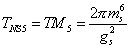
T_NS5 = T_M5 = (2[pi]m_s⁶)/g_s²

Type IIA superstring theory is M-theory compactified on a circle of radius R = g_sl_s, where g_s is the coupling constant, and l_s is the string length. M-theory is a well-defined quantum theory in 11 dimensions, which is approximated at low energy by 11-dimensional supergravity. Its excitations are the massless supergraviton, the M2-brane, and the M5-brane. These account of both the familiar perturbative fundamental string of the IIA theory, and for many of its non-perturbative excitations.

Type IIB superstring theory, which is also an 11-dimensional maximally supersymmetric string theory with 32 conserved supercharges, is chiral, meaning parity violating. At low energy, Type IIB superstring theory is approximated by Type IIB supergravity, similar to how M-theory is approximated by 11d supergravity. Type IIB superstring theory or supergravity has two scalar fields, the dilaton φ, and the axion X. These are combined together to form a complex field

p = X = ie^-[phi]

SL(2, R) is the set of all two-by-two matrices over the real numbers with determinant 1. You can also have SL(2, C) or SL(2, Z). “S” is for special, meaning unitary, determinant 1, “L” is for linear, “2” is a reference to 2 x 2 matrices, “R” is for real numbers, “C” is for complex numbers, and “Z” is for integers. The supergravity approximation has an SL(2, R) symmetry that transforms non-linearly

p -> (ap + b)/(cp + d)

where a, b, c, and d are real numbers satisfying

ad – bc = 1

This is called a Mobius transformation. In the quantum string theory, this symmetry is broken to the discrete subgroup SL(2, Z), which means that a, b, c, and d are integers.

The vacuum value of the p field is

= ([theta]/2[pi]) + i/g_s²

The SL(2, Z) transforms p → p + 1 which implies that θ is an angular coordinate. If θ = 0, then

p -> -1/p

means

g_s = -1/g_s

which is what we’ve been calling S-duality. In Type IIB superstring theory, the coupling constant g_s is the same as the coupling constant 1/g_s, which means that Type IIB theory is self-dual under S-duality. The weak coupling expansion is the same as the strong coupling expansion. S-duality also relates Type I superstring theory to SO(32) heterotic superstring theory.

The name S-duality originates in the fact that the complex field

p = X + ie^-[theta]

that parametrizes SL(2, R)/U(1) was called the superfield S.

Type IIA and Type IIB superstring theories are related by T-duality, meaning if they are compactified on a circle of radii R_A and R_B, then R_AR_B = l_s². Type IIA superstring theory is actually M-theory compactified on a circle. If you combine these two facts together, it turns out that Type IIB superstring theory compactified on a circle, R⁹ x S¹, is equivalent to M-theory compactified on a torus, R⁹ x T².

You could say that all the superstring theories are really one 11-dimensional theory at a fundamental level, so Type IIB superstring theory is really 11-dimensional, say with one dimension compactified on a circle, giving the familiar 10-dimensional theory. Then take that 10-dimensional Type IIB theory, and compactify one of its dimensions on a circle, giving R⁹ x S¹. Then take M-theory, which is obviously 11-dimensional, and compactify two of its dimensions on a torus, giving R⁹ x T². There is a duality between these two theories, and they are related by

m_p³ A_M = ½[pi]R_B

where m_p is the Planck mass, A_M is the area of the torus that two of the dimensions of M-theory are compactified on, and R_B is the radius of the circle that one of the dimensions of Type IIB theory are compactified on. As the radius of the circle gets smaller, the area of the torus gets larger. As the area of the torus gets larger, the radius of the circle gets smaller. As the circle gets larger, the torus gets smaller. As the torus gets smaller, the circle gets larger. You see how this is analogous to T-duality, and therefore, Type IIB theory and M-theory are also one theory.

With S-duality, theory A at strong coupling is equivalent to theory B at weak coupling, and vice versa. If φ is the dilaton field, you have

[phi]_A = -[phi]_B

g_s = e^[phi]

With T-duality, theory A compactified on a space of large volume is equivalent to theory B compactified on a space of small volume, and vice versa. If t is a scalar field other than the dilaton, you have

t_A = -t_B

With U-duality, theory A compactified on a space of large volume is equivalent to theory B at strong coupling. Theory A compactified on a space of small volume is equivalent to theory B at weak coupling. You have

t_A = ±[phi]_B

With each of these dualities, the two theories are really different descriptions of the same theory.

In supergravity theories that represent the low energy effective action for the massless modes of a superstring compactification, you have a non-compact global symmetry group G. The group G is realized non-linearly by scalar fields that parametrize the homogeneous space G/H, where H is the maximal subgroup of G. The first example of this phenomenon, with G = SL(2, R), and H = U(1), was discovered by Cremmer, Ferrara, and Scherk in 1976, in the N = 4 supergravity. A discrete subgroup of symmetry of this particular example corresponds to the S-duality that was first seen in string theory, the toroidally compactified heterotic string. Then an analogous non-compact E₇ symmetry was found in N = 8 supergravity by Cremmer and Julia in 1978. This corresponds to the toroidally compactified Type II string, and combined S, T, and U dualities in a single group.

In 1990, Font suggested that the SL(2, Z) subgroup of SL(2, R) of Cremmer, Ferrara, and Scherk should be the exact same symmetry as the toroidally compactified heterotic string. This proposal extends the duality conjecture of Montona and Olive from supersymmetric gauge theories to superstrings. Let’s look at S duality, which is usually written

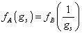
f_A(g_s) = f_B(1/g_s)

This has a subtle similarity to the electric and magnetic fields in an electromagnetic wave, according to classical electromagnetism. For this reason, this sort of reciprocal relationship is sometimes called an electric-magnetic duality. Of course, the name is intended metaphorically.

SO(k, l), where “l” is lower case L, is the non-compact form of SO(k + l) that preserves a metric with k plus signs, and l minus signs. The group SO(k) x SO(l) is its maximal compact subgroup. The quotient space SO(k, l)/SO(k) x SO(l) is a homogenous space of dimension kl. The discrete group SO(k, l; Z) is an infinite group consisting of all SO(k, l) matrices with integer entries. When l = k + 16, it is the subgroup of SO(k, l) that preserves a certain even self-dual lattice of signature (k, l) introduced by Narian. The Narian space M_{k, l} is defined as

M_{k, l} = SO(k, l; Z) \ SO(k, l) / SO(k) x SO(l)

With the toroidial compactification of the heterotic string, no supersymmetry is broken, and in four dimensions, there are 132 scalar fields on the Narian moduli space M_{6, 22}. The T-duality group for the 4d heterotic string is G_T = SO(6, 22; Z). The 132 scalar fields belong to 22 abelian N = 4 gauge multiplets. When you compactify the extra dimensions, 21 of the scalar fields are from the metric, 15 are from the 2-form B_uv, and 96 are from the 16 U(1) gauge fields that form the Cartan subalgebra E₈ x E₈ or SO(32).

The toroidally compactified heterotic string also has two additional scalar fields, the axion, X, and the dilaton, φ, which are in the N = 4 supergravity multiplet. The dilaton is the 10-dimensional dilaton shifted by a function of the other moduli such that the exponential of its vacuum expectation value gives the 4d coupling constant. The 4d axion is the scalar field that is dual to the 2-form B_uv in 4d. The supergravity theory that contains these fields is the same one that was studied by Cremmer, Ferrara, and Scherk. They showed that X and φ parametrize the homogeneous space SL(2, R)/U(1). In the quantum theory, only the discrete S-duality subgroup SL(2, Z) is a symmetry, and the moduli space is

M_s = SL(2, Z) \ SL(2, R) / U(1)

so if you have the following complex scalar field

p = X + ie^-2[phi] = p₁ + p₂

where sometimes the 2 is there as a convention, and the vacuum expectation value is

p = [theta]/2[pi] + i/g_s²

where θ is the vacuum angle, and g_s is the coupling constant, N = 4 Yang-Mills theories have vanishing beta function, so that θ and g_s are well defined independent of scale.

In terms of p, the SL(2, Z) symmetry is realized by non-linear transformations.

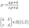
p -> (ap + b)/(cp + d)

When instanton effects are taken into account, the continuous Peccei-Quinn symmetry X → X + b is broken to the discrete subgroup for which b is an integer. This subgroup and the inversion p -> -1/p generate the discrete group SL(2, Z), or when matrices are not distinguished by their negatives, PSL(2, Z). When θ = 0, you have g_s = 1/g_s. The SL(2, Z) symmetry of the theory is broken completely by any specific choice of vacuum. Only when the vacuum expectation value of p is at one of the orbifold points in the moduli space, does some unbroken symmetry, Z₂ or Z₃, remain.

The Type IIA and IIB superstring theory compactification on T⁶ is approximated at low energy by N = 8 supersymmetry. The classical theory has a non-compact symmetry group E_{7, 7}. The duality group is the discrete subgroup E₇(Z), which is the intersection of the continuous E_{7, 7} group and the discrete group Sp(28; Z). In the 56-dimensional fundamental representation, E_{7, 7} is a subgroup of the non-compact group Sp(28). The Narian moduli space is

M = E₇(Z) \ E_{7, 7} / SU(8)

Let’s say you have supersymmetry with N > 1. The extended 4d supersymmetry algebra in 2-component notation includes the anticommutator

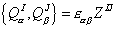
{Q_[alpha]^I, Q_[beta]^J} = [epsilon]_{[alpha][beta]}Z^IJ

The central charges are where Z^IJ = -Z^JI, and the number of central charges is

N(N – 1)/2

where N is the number of the supersymmetry. The central charges are complex numbers whose real and imaginary parts give the electric and magnetic charges associated with the N(N – 1)/2 U(1) gauge fields in the N-extended 4d supergravity multiplet. Therefore, the supersymmetry algebra causes the mass of any state to be bounded below by its central charges. This lower bound is called the Bogomol’nyi bound. When the mass of a state reaches the minimum value allowed for the given charges and moduli, the state is called BPS saturated. BPS states belong to smaller representations of the algebra then are possible when the bound is not saturated. These states are often called BPS branes, named after Bogomol’nyi, Prasad, and Sommerfield.

Let’s look at the N = 4 supersymmetry. You have

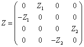
In the N = 4 case, even though the supergravity multiplet has six U(1) gauge fields, you can describe a generic configuration by only describing two electric and two magnetic states. There are two ways to achieve BPS saturation. In the first way, the mass satisfies the following relation

M = | Z₁ | = | Z₂ |

This gives ultrashort multiplets, such as the 16-dimensional gauge multiplet. The second way to create a BPS state is if you have

M = | Z₁ | > | Z₂ |

The first scenario takes place when the electric charge vector α^a and the magnetic charge vector β^a are parallel. The second scenario takes place when they are not parallel. Since the BPS states in the perturbative string spectrum are purely electric, they are therefore of the first type.

This actually allows you to make comparisons between string states and black holes. Static extremal black hole configurations with

M = | Z₁ | = | Z₂ |

turn out to preserve one half of the supersymmetry, and have a horizon of vanishing area, and thus no Berkenstein-Hawking radiation. Static extremal black hole configurations with

M = | Z₁ | > | Z₂ |

preserve only one fourth of the supersymmetry, and have a horizon of finite area. Let’s say you have N = 8 supersymmetry. In that case, in order to obtain a finite area horizon, M would have to be equal to only one of the four | Z_i |’s, so that 7/8 of the supersymmetry is broken, and only 1/8 is preserved. This allows you to measure the entropy of supersymmetric black holes with finite area horizons by counting the number of microscopic string degrees of freedom.

Let’s look at M-theory in more detail. In 1978, Cremmer, Julia, and Scherk developed 11-dimensional supergravity which was non-renormalizable and did not admit compactifications. It turned out that Type IIA superstring theory is the dimensional reduction of d = 11 supergravity. The 2-form potential of d = 10 supergravity is associated with a string. The 3-form potential of d = 11 supergravity is associated with a membrane. While it was known how to incorporate spacetime supersymmetry into string theory using the Green-Schwarz world sheet action, it was not known how to generalize this to higher dimensional objects. They were able to solve this problem by looking at d = 4 theories that were actually dimensional reductions from higher dimensional theories. It was known that the d = 4 Green-Schwarz action could be interpreted as the effective action for Nielson-Olesen vortices in a N = 2 supersymmetric abelian Higgs model, which is actually a dimensional reduction to d = 4 from d = 6, and where the vortices are what we would now call D3-branes. The effective action for this d = 4 D3-brane is a higher dimensional generalization of the Green-Schwarz action, which is exactly what we were looking for. This pointed the way to a construction by E. Bergshoeff, E. Sezgin, and P. K. Townsend in 1988, of a d = 11 supermembrane action, and the interpretation of d = 11 supergravity as the effective field theory of a hypothetical supermembrane theory. It was later showed that the Green-Schwarz action for the Type IIA superstring is the dimensional reduction of the d = 11 supermembrane action. This suggested an interpretation of the Type IIA superstring as a membrane wrapped around the 11th dimension which had been compactified on a circle. In 1994, M. J. Duff, K. S. Stelle, G. W. Gibbons, and P. K. Townsend constructed an extreme membrane solution of d = 11 supergravity, and showed that it reduces in d = 10 to the extreme string solution of type IIA supergravity, which had been earlier identified as the field theory realization of the Type IIA string.

Now at this point, the connections between d = 10 and d = 11 physics were still classical. It still seemed unrealistic that the quantum IIA superstring theory, with d = 10 as its critical dimension, could be 11-dimensional. In addition, the non-renormalizability of d = 11 supergravity appeared to have been simply replaced by the difficulty of a continuous spectrum for the first quantized supermembrane. However, the inclusion of wrapping modes of the membrane and 5-brane led to a spectrum of solitons identical to that of the IIA string if the latter includes the wrapping modes of the d = 10 p-branes carrying Ramond-Ramond charges. However, if this is to be taken to mean that IIA superstring theory really is 11-dimensional, then its non-perturbative spectrum in d = 10 must include the Kaluza-Klein excitations from d = 11. These would have long range 10-dimensional fields, and so would have to appear as BPS-saturated 0-brane solutions of IIA supergravity. Such solutions, and their 6-brane duals, were already known to exist, and they were then interpreted as field realizations of the Kaluza-Klein modes, and the Kaluza-Klein 6-branes needed for the d = 11 interpretation of Type IIA superstring theory.

Because of the connection between the string coupling constant and the dilaton, it was obvious that you needed a better understanding of the dilaton in order to formulate a non-perturbative string theory. The fact that type IIA supergravity is the dimensional reduction of d = 11 supergravity, leads to an interpretation of the dilaton as a measure of the radius of the circle that the 11th dimension is compactified on. This leads to the following relation.

R₁₁ = g_s^2/3

where R₁₁ is the radius of the circle that the 11th dimension of M-theory is compactified on.

This shows that a power series in g_s is an expansion about R₁₁ = 0, so that the 11th dimension would go to zero radius, and not be detectable in string perturbation theory. This connection between the string coupling constant and the radius of the compactified 11th dimension could have been used earlier if people had thought of it. The reason they did not is because the area of the wrapped brane, and thus its energy, is proportional to R₁₁. This implied that the tension of the membrane would vanish in the R₁₁ → 0 limit. The reason this does not happen is because the energy as measured in d = 10 superstring theory differs from that measured in d = 11 by a factor of R₁₁, which is such as to ensure that the d = 10 string tension is independent of R₁₁, and therefore non-zero in the R₁₁ → 0 limit. This also ensures that the 0-brane mass is proportional to 1/R₁₁, which you need for its interpretation as a Kaluza-Klein excitation. In the strong coupling limit, R₁₁ goes to infinity, the vacuum is 11-dimensional Minkowski, and the effective field theory is 11-dimesional supergravity.

Let’s look at how you get a chiral theory like Type IIB superstring theory from a compactification of M-theory. This is a specific example of the general problem of how do you get chiral theories from compactifying d = 11 supergravity. There are two ways to do this. The first way uses the fact that you can consider compactifications of M-theory on orbifolds. The second way, which is what’s used for Type IIB string theory, is that chiral theories can emerge as limits of non-chiral theories as a result of massive modes not present in the Kaluza-Klein spectrum. Let’s say you have d = 11 supergravity compactified on T². You have d = 9 N = 2 supergravity coupled to a KK tower of massive spin-2 multiplets. In the limit where the surface area of the torus goes to zero, keeping the shape the same, you get the non-chiral d = 9 supergravity theory. If you have M-theory compactified on T², you also have massive spin-2 multiplets coming from membrane wrapping modes on T². Those additional massive modes become massless in the limit of the area of the torus going to zero, in such a way so that the effective theory of resulting massless fields is the 10-dimensional chiral Type IIB supergravity. Since this is a chiral theory, there are two versions of it, either right-handed or left-handed. Which one you get depends on the sign of the Chern-Simons term in the d = 11 supergravity Lagrangian, or on the sign of the Wess-Zumino term in the supermembrane action. Therefore, M-theory includes a mechanism that allows for the emergence of chirality upon compactification.

A torus has two radii. Let’s say one is the radius of the 10th dimension, R₁₀, and the other radius of the torus is the radius of the 11th dimension, R₁₁, so the 10th and 11th spacetime dimensions are compactified on a torus.

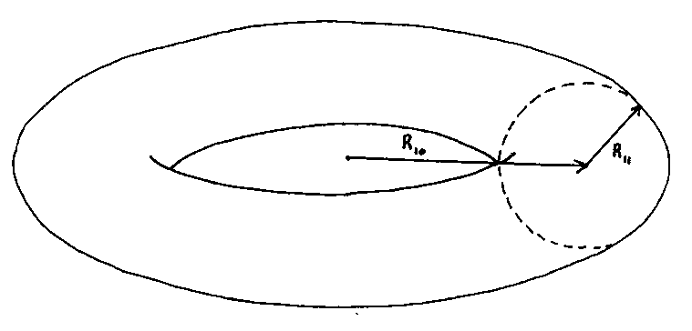
If you look at the limit

R₁₀ -> [infinity]

at fixed R₁₁, you end up with Type IIA theory, with coupling constant

g_sA = R₁₁^3/2

where g_sA is coupling constant of Type IIA superstring theory. Now, remember that Type IIA and Type IIB superstring theory are T duals. Type IIA theory is equivalent to Type IIB theory compactified on a circle of radius 1/R₁₀. It follows that the S¹-compactified IIB theory can be understood as T²-compactified M-theory. If you look at the limit

R₁₁ -> 0

R₁₀ -> 0

at fixed ratio, you end up with uncompactified IIB theory with string coupling constant

g_sB = R₁₁/R₁₀

where g_sB is the coupling constant of IIB theory.

The interchange of R₁₀ and R₁₁ is simply a reparametrization of the torus. In other words, the IIB theory at coupling g_sB is equivalent to IIB theory at coupling 1/g_sB. More generally, the discrete SL(2, Z) group of global reparametrizations of the torus implies an SL(2, R) symmetry of the IIB theory, originally proposed on the basis of the SL(2, R) symmetry of IIB supergravity. The following diagram of moduli space shows how Type IIA, Type IIB, and M-theory are related through T² compactification.

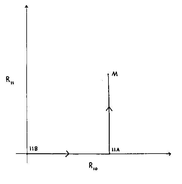
So if you start with Type IIB theory, and increase R₁₀, you end up with Type IIA theory. Then if you have Type IIA theory, and increase R₁₁, you end up with M-theory. A generic point on this diagram refers to an 11-dimensional vacuum. If R₁₁ = 0, and R₁₀ → 0, you have free string theories. (R₁₀, R₁₁) = (0, 0) corresponds to the uncompactified IIB superstring theory for which the vacuum is 10-dimensional Minkowski spacetime. (R₁₀, R₁₁) = (0, 0) is not really a point in the moduli space because the IIB coupling constant depends on how the (R₁₀, R₁₁) → (0, 0) limit is taken. The Type IIA theory has a straightforward interpretation as M-theory compactification.

The S¹ compactified IIB theory belongs to the same moduli space as the T²-compactified M-theory. How does the d = 11 membrane emerge from IIB theory? The Type IIB theory is not just a theory of strings, but also contains M3-branes. If during S¹-compactification, the M3-brane wraps around the circle, it becomes an M-theory membrane. However, what if it does not wrap around the circle? You then have to find this M3-brane in M-theory. The uncompactified M-theory is not just a theory of membranes, but also includes M5-branes. If upon T²-compactification, an M5-brane wraps around the torus, it appears as an M3-brane. Of course, the M5-brane could also not wrap around the torus. You then end up with both M3-branes and M5-branes in all the different compactifications. Here we are using Mp-brane to mean a Dp-brane within the spectrum of M-theory, and using membrane to mean a D2-brane.

From the description of IIB superstring theory as a limit of a T²-compactified M-theory, the complex structure of the torus, viewed as a Riemann surface, will survive the limit to become a parameter determining the choice of IIB vacuum. This parameter is the vacuum value of the complex IIB supergravity field

p = X + ie^-[theta]

where φ is the dilaton, and X is the axion. If p were assumed to be single-valued in the upper half plane, then it would have to be constant over the complex KK space in any compactification of the IIB theory.

However, p actually takes values in the fundamental domain of the modular group of the torus, so it doesn’t have to be single-valued in the upper half plane. A class of compactifications that takes advantage of this possibility is called F-theory.

F-theory is a hypothetical 12-dimensional theory. 11d supergravity, and thus M-theory, can be compactified on a Ricci-flat four dimensional K₃ manifold. For some Ricci-flat metrics, K₃ can be viewed as an elliptic fibration of CP¹, meaning as a fiber bundle where the fiber is a torus whose complex structure p varies over a Riemann sphere. Generically, there will be 24 singular points on the Riemann sphere at which the torus degenerates, but these are merely coordinate singularities as long as no two singular points are in the same place. Thus, there exists M-theory compactifications on manifolds that are locally isomorphic to T² x S². If the 2-torus is then shrunk to zero area, you get an S² compactification of the IIB theory in which the scalar field p varies over S². More generally, given a Ricci-flat manifold E that is an elliptic fibration of a compact manifold B, you can define F-theory on E as IIB theory on B with p varying over B in a way proscribed by its identification as the complex structure of the torus in the description of E as an elliptic fibration. F-theory would then be a 12-dimensional theory.

Let’s now look at the two heterotic string theories. The two heterotic strings have d = 10 N = 1 supersymmetry, and are related to each other by T-duality, at least to all orders in perturbation theory. The compactification of either theory on a circle allows a non-vanishing Wilson line, the integral of A, around the circle, where A is the Lie algebra valued gauge field of the effective supergravity and Yang-Mills theory. You are essentially choosing a non-zero expectation value for the component A in the compact direction. The expectation value must lie in the Cartan subalgebra of either SO(32) or E₈ x E₈. The gauge group is broken to SO(16) x SO(16). A SO(16) x SO(16) heterotic string theory obtained by compactification of the SO(32) heterotic string on a circle of radius R can also be obtained by compactification of the E₈ x E₈ theory on a circle of radius 1/R. Therefore, the uncompactified SO(32) and E₈ x E₈ heterotic string theories are theories with vacua that are limiting points in a single connected space of vacua. SO(32) and E₈ x E₈ heterotic strings are related by T-duality. SO(32) heterotic and Type I string theories are related by S-duality. It turns out that Type I string theory can be derived from Type IIB string theory.

Let’s look at Type I string theory. Type I string theory is an orientifold of Type IIB theory. The Type IIB string action is invariant under a world sheet parity operation called Ω which exchanges left-movers and right-movers. You can therefore find a new string theory by gauging this symmetry. This projects out the world sheet parity odd states of the Type IIB superstring theory, leaving the states of the closed string sector of Type I theory. This sector is anomalous by itself but you can add an open string sector which can be viewed as an analog of the twisted sector in more conventional orbifold construction. An anomaly free theory can then be obtained by including SO(32) Chan-Paton factors at the ends of the open strings. This is Type I string theory. From its origin in IIB theory, it is obvious that the S¹-compactified Type I string must be 11-dimensional. Since the IIA theory has a more direct connection to d = 11 then IIB, and IIA is the T-dual of IIB, it is logical to expect that the connection between Type I and d = 11 will be more obvious if you consider its T-dual. The T-dual of Type I string theory is called Type IA or Type I’ theory.

To explain Type IA theory, let’s first look at Type I theory in which the SO(32) gauge group is broken to SO(16) x SO(16) by the inclusion of Wilson lines. Let’s say you have

Y(t, [sigma])

which is the map from the string world sheet to the circle. T-duality exchanges Y for its world sheet dual [Y tilda]. Since Y is a world sheet scalar, [Y tilda] is a pseudoscalar.

[omega] [[Y tilda]](t, [sigma]) = -[Y tilda](t, -[sigma])

Let [y tilda] be the constant in the mode expression of Y(σ), then

[omega][[y tilda]] = -[y tilda]

The gauging of world sheet parity means that a point on the circle with coordinate [y tilda] is identified with the point with coordinate -[y tilda] so the circle becomes an orbifold S¹/Z₂, where the Z₂ action has two fixed points at

[y tilda] = 0, [pi]

Since S¹/Z₂ is just the closed interval

I = [0, [pi]]

the fixed points are actually 8-plane boundaries of the 9-dimensional space, called orientifold planes because the Z₂ action on S¹ is coupled with a change of orientation on the world sheet.

Therefore, the Type IA theory is effectively Type IIA theory compactified on the orbifold S¹/Z₂, which is like a circle containing a singularity because if you define one point on the circle to be the beginning, that point is also the end of the line segment. Closed strings that wind around the circle become open strings stretched between two 8-plane boundaries, each of which is associated with an SO(16) gauge group. Actually, the open strings in Type IA theory do not end on the 8-planes themselves but instead on 8-branes which coincide with them. Since a IIA superstring is a S¹-wrapped supermembrane in d = 11 spacetime, the open strings of the IA theory must be wrapped d = 11 supermembranes stretched between two S¹-wrapped 9-plane boundaries in d = 11 spacetime. Let L be the distance between these boundaries, and R be the radius of the circular dimension. Then you can identify Type IA theory as the R → 0 limit of M-theory compactified on a cylinder of radius R and length L. The stretched membrane is effectively wrapped on the cylinder, and has a closed string boundary on each of the two S¹-wrapped 9-plane boundaries. Each string boundary must carry an SO(16) current algebra in order that an SO(16) gauge theory will emerge in the R → 0 limit.

Here you can draw the following moduli space.

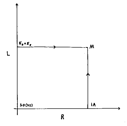
This shows the relation between Heterotic SO(32), Heterotic E₈ x E₈, Type IA string theory, and M-theory, where R is the radius of the cylinder, and L is the length of the cylinder. The moduli space of M-theory compactified on a cylinder includes all superstring theories with N = 1 supersymmetry. The generic vacuum of this moduli space is 11-dimensional, but you get a 10-dimensional theory with gauge group SO(32) in the limit where both the radius and the length of the cylinder go to zero, so the cylinder shrinks to zero area.

Let’s look at open strings in Type IA theory. T-duality exchanges the Neumann boundary conditions on Y at the ends of an open string with Dirichlet boundary conditions on [Y tilda].

[partial derivative]_t [Y tilda](t, 0) = 0

[partial derivative]_t [Y tilda](t, [pi]) = 0

Therefore, the open strings must now start at some fixed value of [Y tilda], and end at some other, or the same, fixed value. For instance, open strings have their ends tethered to some number of parallel 8-branes. Unlike Neumann boundary conditions, Dirichlet boundary conditions do not prevent the flow of energy and momentum off the ends of the strings, so the 8-branes on which the strings end must be dynamical objects. They are called D-branes. The open strings end on D8-branes. The N = 2 supersymmetry of the IIB theory is broken to N = 1 in the Type I theory because of the restriction on the IIB fermion fields at the ends of open strings. The N = 2 supersymmetry of the IIA theory is also broken to N = 1 in the Type IA theory, but with the difference that since the ends of the open strings lie in the D8-branes, it is only on these branes that the N = 2 supersymmetry is broken. Everywhere else, you have the unbroken N = 2 supersymmetry of IIA theory. Thus, the Type IA theory is equivalent to the IIA theory on an interval with some number of D-branes.

The supersymmetry algebra implies a bound on the mass, for fixed charge, that is typically saturated. The state is then called BPS-saturated. BPS-saturated states preserve some fraction of the supersymmetry of the vacuum. The force between static BPS-saturated states vanishes so there also exist static BPS-saturated multi-soliton solutions. There is a generalization of this to Type II supergravity theories in which a multi-soliton is identified with a solution representing a number of parallel infinite planar p-branes. The central charge in the supersymmetry algebra becomes a p-form charge. Some of these p-branes, which all preserve half the d = 11 N = 2 supersymmetry, carry the charges associated with (p + 1)-form gauge potentials coming from the Ramond-Ramond, or R x R, sector of the Type II superstring theory. They are the R x R branes. There are R x R p-branes of IIA supergravity, for which p = 0, 2, 4, 6, and 8. There are R x R p-branes of IIB supergravity, for which p = 1, 3, 5, and 7. For p-branes in general, the long wavelength dynamics is determined by effective (p + 1)-dimensional field theory. For R x R branes, this world volume field theory includes a U(1) gauge potential. This is because the R x R branes of Type II supergravity theories are the field theory realization of the Type II superstring D-branes. This allows a string theory computation of the bosonic sector of the effective world volume field theory. The full action is then determined by supersymmetry and kappa symmetry. The result, upon partial gauge fixing, is a non-linear supersymmetric U(1) gauge theory of the Born-Infeld type, except that the fields now depend on the (p + 1) world volume coordinates of the brane.

Let’s construct the M-theory superalgebra. This is similar to before when I constructed the GS action of superstring theory. If you like, you can reread the section on the GS formalism of superstrings. Let’s first look at the d = 11 supermembrane. In d = 11, the minimal algebra is spanned by the 11-momentum P_M, and a 32 component Majorana spinor of the d = 11 Lorentz group, Q_α, obeying the anticommutation relation

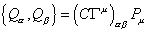
{Q_[alpha], Q_[beta]} = (C[capital gamma]^u)_{[alpha][beta]} P_u

where Q is a Majorana spinor, C is an antisymmetric real charge conjugation matrix, and Γ^u are the Dirac matrices. As before, you introduce the supertranslation invariant 11-vector-valued 1-form on the superspace

[capital pi]^M = dx^M – i[theta bar][capital gamma]^Md[theta]

You next determine the super-Poincare invariant closed forms on the superspace. The only possibility is the 4-form

h₍₄₎ = [capital pi]^M[capital pi]^N d[theta bar][capital gamma]_MN d[theta]

which leads to a membrane rather than a string. I’ll use the word membrane to mean a 2-brane, although some people use it to mean any p-brane. The Nambu-Goto action has an obvious generalization to the p-brane case. The p = 2 case is sometimes called the Dirac action. The p = 2 Nambu-Goto action is

S_D = -[integral] d³ [xi] [squareroot of -det([capital pi]_i . [capital pi]_j)]

There is a k-invariant supermembrane action of the form

S = S_D + S_WZ

where S_WZ is constructed from the 3-form b₍₃₎, where h₍₄₎ = db₍₃₎. Like before with the heterotic and type II superstrings, the WZ term modifies the supersymmetry algebra. Here you have

{Q_[alpha], Q_[beta]} = (C[capital gamma]^M)_{[alpha][beta]} P_M + (C[capital gamma]_MN)_{[alpha][beta]} Z₍₂₎^MN

where Z₍₂₎ is a 2-form charge. You can take this d = 11 supertranslation algebra, and write it as a d = 10 algebra by splitting the charges into their representations under the d = 10 subgroup of the d = 11 Lorentz group. The d = 11 supersymmetry charge becomes a d = 10 Majorana spinor charge, and

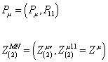
P_M = (P_u, P₁₁)

Z₍₂₎^MN = (Z₍₂₎^uv, Z₍₂₎¹¹ = Z^u)

In this notation, the supersymmetry algebra can be written as

{Q_[alpha], Q_[beta]} = (C[capital gamma]^u)_{[alpha][beta]} P_[alpha] (C[capital gamma]^u)_{[alpha][beta]} Z_u + (C[capital gamma]¹¹)_{[alpha][beta]} + (C[capital gamma]_uv)_{[alpha][beta]} Z₍₂₎^uv

where Γ¹¹ is the product of the Dirac matrices. Notice that not only do you have the 1-form charge Z associated with the IIA string, but you also have a 0-form charge P₁₁, and a 2-form charge Z₍₂₎. This suggests not only that the IIA superstring is really a d = 11 supermembrane but that the non-perturbative d = 10 theory is a theory not just of strings but also 0-branes and 2-branes.

It turns out that a closed (p + 2)-form on superspace is necessary only if, after gauge-fixing the κ-symmetry, the world volume fields consist only of scalars and spinors. While this is the case for p-brane solutions of flat space field theories, and for some p-brane solutions of supergravity theories, it is not true in general, which was originally discovered by an analysis of the small fluctuations about 5-brane solutions of type II supergravity theories. An example in d = 10 are D-branes, whose world volume field content is that of d = 10 vector multiplets dimensionally reduced to (p + 1) dimensions. Another example is the 5-brane solutions of d = 11 supergravity for which the field content is that of 6-dimensional antisymmetric tensor multiplet. These additional possibilities for p-branes in d = 10 and d = 11 supergravity theories are also associated with p-form extensions of the supersymmetry algebra. For instance, the d = 11 super-5-brane is associated with a 5-form extension of d = 11 supergravity algebra. Therefore, the full d = 11 supertranslation algebra is

{Q_[alpha], Q_[beta]} = (C[capital gamma]^M)_{[alpha][beta]} P_M + (C[capital gamma]_MN)_{[alpha][beta]} Z₍₂₎^MN + (C[capital gamma]_MNPQR)_{[alpha][beta]} Z₍₅₎^MNPQR

The three types of charge appears on the right-hand side are those associated with the supergraviton, the supermembrane, and the super-5-brane, which are the three components of M-theory. Therefore, this is the M-theory superalgebra.

Another question is why are some dimensions compactified and others not. In general relativity, the curvature of spacetime is determined by gravity. Since string theory incorporates general relativity, the geometry of spacetime is determined dynamically. This explains how in string theory, which includes gravity, some of the dimensions could be compactified. Gravitational interactions could cause the extra dimensions to be compactified. This was one of the original motivations for why John Schwarz first applied string theory to a possible theory of gravity, since the earlier hadronic theory of strings, which did not include gravity, did not have any explanation as to how or why the extra dimensions could be compactified. However, perhaps a more useful way of phrasing it is to say that gravitational interactions affect the curvature of spacetime in such a way as to prevent dimensions from being compactified. One possibility is that it is the interaction between strings or p-branes that keeps the dimensions from compactifying. Let’s say right after the Big Bang, all the dimensions were non-compact. If all the 11 dimensions were non-compact, and the 10 spatial dimensions were as infinite as the three we’re familiar with, then they would have so much extra room or degrees of freedom, that the strings or p-branes would usually just sail right past each other without interacting. This lack of interaction could cause the dimensions to compactify one by one until you are left with the three uncompactified spatial dimensions we’re familiar with. At that point, there would be little enough room for them to move around in, that interactions would be frequent enough that no further spatial dimensions would compactify.

A related idea is to use the anthropic principle. Let’s say in different parts of the Universe, you had different numbers of dimensions compactified. You could also imagine there being an infinite, or very large, number of universes, and they had different numbers of dimensions, or different numbers of dimensions compactified. If in a given universe, or part of the Universe, there were more than three uncompactified spatial dimensions, the strings or p-branes would usually sail right past each other without interacting. With such a low rate of interaction between particles, it’s unlikely that you would have the large amount of very complex interactions necessary for life to arise. On the other hand, if there were only one or two spatial dimensions, there would be such little room that the particles would crowd each other out, which would make complex interactions more difficult. It is less likely you would have really complex reactions or really complex molecules like DNA. Therefore, you can logically argue that three is the optimum number of uncompactified spatial dimensions for life to arise. Also, planets could not be in stable orbits around stars in more than three spatial dimensions. Also, in more dimensions, there would be more electron-positron pairs surrounding an electron, and thus more charge screening, and so the electromagnetic coupling constant would be less. This is not to say that you couldn’t have life with other numbers of uncompactified spatial dimensions, but it would be less likely. Thus, we aren’t looking at a totally unbiased random sample of universes or parts of the Universe, since we’re here to ask the question. Therefore, you can explain the number of uncompactified dimensions using anthropic arguments.

This is also similar to the Brandenberger-Vafa mechanism. Robert H. Brandenberger and Cumrun Vafa considered what would happen to a tiny universe which is compact in all directions and filled with strings, some of which wind around the compact dimensions. Since the energy of a massive string is roughly proportional to its length, the winding modes of the strings make it expensive to inflate a dimension with winding modes and hence it is natural to assume that dimensions with winding modes stay small, while the rest may expand. Initially all directions have winding modes. However, when a winding string hits another string that winds in the same dimension but in the opposite direction, they may interact and unwind. Using thermodynamics, you then assume that as long as the strings can interact freely they thermalize, which leads to a net zero winding. A one dimensional object is likely to meet another such object only in up to three spatial dimensions. In more spatial dimensions, the probability for winding annihilation decreases drastically. Therefore, thermalization is expected to only happen in three of the available dimensions, which then can grow large while the rest are kept small by winding strings. After branes were discovered/invented, they reconsidered it and extended it to a gas of arbitrary p-branes. This is easily done by noting that a p-brane is likely to meet another p-brane in up to 2p+1 dimensions. For p = 1, this reproduces the above argument. So with various p-branes, the BV mechanism gives rise to a hierarchy of smaller and larger dimensions.

Historically, an important milestone on the road towards M-theory was Seiberg-Witten theory, which opened the door to discussing superstrings non-perturbatively. Nathan Seiberg and Edward Witten did important work on N = 2 supersymmetry. It was followed by Hull and Townsend’s work on heterotic type II string equivalence. The main result of Seiberg-Witten theory was that you could state the exact non-perturbative low energy effective Lagrangian of N = 2 supersymmetric Yang-Mills theory with gauge group SU(2). It contains the effective renormalized gauge coupling g, and the theta angle [theta].

[theta]a/[pi] + 8[pi]i/g²(a) = 8[pi]i/g₀² + 2i/[pi] log [a²/[capital lambda]²] – i/[pi] [summation over l from 1 to infinity] c_l ([capital lambda]/a)^4l

where Λ is the dynamically generated scale at which gauge coupling becomes strong, a is the Higgs field, g is the gauge coupling, c_l is the instanton coefficients, and “l” is lower case L. The first term on the right-hand side is the bare value. The second term is the one loop effects. The third term is the instanton effects. The instanton effects is what causes non-perturbative effects. The difficulty in calculating non-perturbative effects is that you don’t know the instanton coefficients c_l. It was the achievement of Seiberg and Witten to determine all of the instanton coefficients c_l explicitly. These coefficients give infinitely many predictions for zero momentum correlators involving a and gauginos in non-trivial instanton backgrounds. These correlators are topological. The fact that highly non-trivial mathematical results can be reproduced was striking evidence that Seiberg and Witten’s approach was correct.

A recent development called Matrix theory, developed by Tom Banks among others, enables you to confirm many of the predictions of M-theory. You can prove the dualities and other relationships among the theories. Matrix theory is constructed in terms of N points, actually D0-branes, which exist in the 11-dimensional spacetime. The D0-brane is a BPS-state, and has a mass of

1/g_sl_s

Their spatial positions are determined by the eigenvalues of nine N x N matrices, where N is eventually taken to infinity. The 10th dimension depends on N, the number of points. The 11th dimension lies on the light cone. Therefore, you only have nine dimensions left to be specified by matrix eigenvalues. So you see how you have reduced the number of dimensions you have to specify by one since the 10th dimension is determined by N. This is an example of a concept called the holographic principle where the physics of d-dimensional space, say 3d space, is determined by its (d – 1)-dimensional boundary, such as the 2d surface of 3d space. In this case, you can describe 10-dimensional space by only specifying nine dimensions. The light cone construction has its origin in the idea first thought of by Leonard Susskind and Gerard ‘t Hooft that the three-dimensional space in which we live can be completely described by its two-dimensional boundary because the third dimension is not independent of the other two dimensions. Tom Banks advocates the view that Matrix theory is in fact the fundamental M-theory. The construction has a generalization that describes compactification of M-theory on a torus, Tⁿ. Although it’s promising, there still remain problems with Matrix theory. It does not seem to work for n > 5. It treats the 11th dimension differently from the other dimensions.

Matrix theory is formulated in the light cone frame. It is constructed by building an infinite momentum frame, or IMF, boosted along a compact direction by starting from a frame with N unites of compactified momentum, and taking N to infinity. Lorentz invariance will arise, if at all, only in the large N limit. Therefore, Matrix theory is not background independent. A complete list of allowed backgrounds has not yet been found. Many properties of Matrix theory appear to be connected with noncommutative geometry. In the current formation of Matrix theory, gravity and geometry emerge in a very awkward fashion.

You take general ideas of holographic theories in the infinite momentum frame, and combine them with maximal supersymmetry, and you get a unique Lagrangian for the fundamental degrees of freedom in flat infinite 11-dimensional spacetime. The quantum theory based on this Lagrangian contains the Fock space of 11-dimensional supergravity, as well as metastable states representing large semiclassical membranes. Charles Thorne suggested an approach to nonperturbative string theory based on the idea of string bits. Light cone gauge string theory can be viewed as a parton model in the IMF along a compactified spacelike dimension whose partons or fundamental degrees of freedom, carry only the lowest allowed value of the longitudinal momentum. In perturbative string theory, this property follows from the fact that longitudinal momentum is the length of the string in the IMF. Susskind realized that this property of string theory suggested that string theory obeyed the holographic principle, which had been proposed by ‘t Hooft as the basis of a quantum theory of black holes. The ‘t Hooft-Susskind holographic principle states that the fundamental degrees of freedom of a consistent quantum theory including gravity must live on a (d – 2)-dimensional transverse slice of d-dimensional spacetime. This is equivalent to saying they carry only the lowest value of longitudinal momentum so that wavefunctions of composite states are described in terms of purely transverse coordinates. This requires supersymmetry in order to work.

You construct a holographic IMF theory by taking the limit of a theory with a finite number of degrees of freedom. The Super-Galilean algebra consists of transverse rotations, J^ij, transverse boosts, Kⁱ, and supergenerators. Aside from the rotational commutators, the Super-Galilean algebra has the following form.

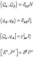
{Q_[alpha], Q_[beta]} = [delta]_{[alpha][beta]} H

{q_[alpha], q_[beta]} = [delta]_AB P_L

[Q_[alpha], q_A] = [gamma]_A[alpha]ⁱ P_i

[Kⁱ, P^j] = [delta]^ij P⁺

Since there are 11 spacetime dimensions, there are 9 transverse dimensions. The 10th spatial direction is the longitudinal direction of the IMF. We imagine it to be compact, with radius R. The total longitudinal momentum is N/R. The Hamiltonian is the generator of translations in light cone time, which is the difference between the IMF energy, and the longitudinal momentum. The essential simplification of the IMF follows from thinking about the dispersion relations for particles.

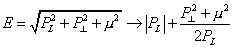
E = [squareroot of P_L² + P_{[perpendicular]}² + M²] -> | P_L | + (P_{[perpendicular]}² + M²)/2 P_L

The second form of this equation is exact in the IMF. It shows that particle states with negative or vanishing longitudinal momentum are eigenstates of the IMF Hamiltonian, E – P_L, with infinite eigenvalues. You can then integrate them out, leaving a local in time Hamiltonian formulation of the dynamics of those degrees of freedom with positive longitudinal momenta.

The dynamical SUSY algebra is very difficult to satisfy. The known representations of it are all theories of free particles. To obtain interacting theories, you have to generalize the algebra to

{Q_[alpha], Q_[beta]} = [delta]_{[alpha][beta]} + Y^A G^A

where G^A are generators of a gauge algebra which annihilate physical states.

If the degrees of freedom transform in the adjoint representation of the gauge group, the SUSY generators are linear in the canonical momenta of both Bose and Fermi variables, and there are no terms linear in the bosonic momenta of the Hamiltonian, then the unique representation of this algebra with a finite number of degrees of freedom is given by the dimensional reduction of the 9 + 1 dimensional SUSY Yang-Mills to 0 + 1 dimensions. The Super-Galilean symmetry, with kinematical SUSY generators is given by

q_[alpha] = Tr [theta]_[alpha]

where θ_α are the fermionic superpartners of the gauge field.

In order to have a Lagrangian where the number of the degrees of freedom is arbitrarily large, you can only have the groups U(N), O(N), or Sp(2N). However, the only one that is actually realized is U(N). The orthogonal and sympletic groups only appear in situations with reduced supersymmetry.

Duff, Hull, Townsend, and Witten established the existence of M-theory. Witten studied states that are charged under the Ramond-Ramond one-form gauge symmetry. The fundamental charged object is a D0-brane whose mass is

1/g_sl_s

D0-branes are BPS states. If you assume the existence of a threshold bound state of N of these particles, and take into account the degeneracies implied by SUSY, you get a spectrum of states equivalent to that of 11d supergravity compacified on a circle of radius R = g_sls.

If the Type IIA/M-theory duality is correct, the momentum in the tenth spatial dimension is identified with Ramond-Ramond charge, and is carried only by D0-branes and their bound states. If you take the D0-branes to be fundamental constituents, then they carry only the lowest unit of longitudinal momentum. In an arbitrary reference frame, you also have anti-D0-branes, but in the IMF, the only low energy degrees of freedom will be positively charged D0-branes. You go to the IMF by adding N D0-branes, and taking N to infinity.

One of the most important advances in superstring theory in recent years is Anti-de Sitter/Conformal Field Theory, or AdS/CFT correspondence, discovered by Juan Maldacena in 1997, and made more precise by Gubser, Klebanov, Polyankov, and independently by Witten, in 1998. This is an equivalence between superstring theory on certain ten-dimensional backgrounds involving Anti-de Sitter spacetime, and four-dimensional supersymmetric Yang-Mills theories. The AdS/CFT correspondence is very surprising because it relates a theory of gravity to a theory with no gravity at all, and no particles with spin > 1, and it relates highly non-perturbative problems in Yang-Mills theory to problems in classical superstring theory or supergravity. Also, it relates a ten-dimensional theory to a four-dimensional theory, so it involves the holographic principle. Aside from being surprising, it is also very useful. The reason this is useful is because a problem that is difficult on one side of the correspondence, might be easy to solve on the other side. Therefore, you can convert difficult problems into easy problems.

The AdS/CFT correspondence suggests an amazing equivalence between two seemingly unrelated theories. On the AdS side of the correspondence, you have 10-dimensional Type IIB superstring theory compactified on the product space of 5-dimensional Anti-de-Sitter space and a five-sphere, AdS₅ x S⁵, where the Type IIB 5-form flux through S⁵ is an integer N, and the AdS₅ and S⁵ have equal radii L given by

L⁴ = 4[pi]g_sN[alpha]’

On the other side, the SYM side, of the correspondence, you have 4-dimensional supersymmetric Yang-Mills theory with maximal N = 4 supersymmetry, gauge group SU(N), and Yang-Mills coupling g_YM² = g_s in the conformal phase. The AdS/CFT conjecture states that these two theories, including operator observables, states, correlation functions, and full dynamics are equivalent to each other.

In the strongest form of the conjecture, the correspondence is to hold for all values of N, and all regimes of coupling g_s = g_YM². It’s also useful to look at certain limits of the conjecture. The ‘t Hooft limit of the SYM-side, in which

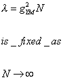
[lambda] = g_YM² N

is fixed as N → ∞ corresponds to classical string theory on AdS₅ x S⁵, with no string loops on the AdS side. Therefore, classical string theory on AdS₅ x S⁵ provides with a classical Lagrangian formulation of the large N dynamics of N = 4 SYM theory, called the masterfield equations. A further limit λ → ∞ reduces classical string theory to classical Type IIB supergravity on AdS₅ x S⁵. Therefore, strong coupling dynamics in SYM theory, at least for the large N limit, is mapped onto classical low energy dynamics in supergravity and string theory, which is much easier to solve. You have a correspondence between a 10-dimensional theory of gravity, and a 4-dimensional theory with no gravity at all, and no particles with spin > 1.

The original correspondence by Juan Maldacena is between N = 4 SYM in its conformal phase, and string theory on AdS₅ x S⁵. You can also use AdS₆ x S⁴ or AdS₄ x S⁶. The conjecture can also be adapted to situations without conformal invariance, and with little or no supersymmetry on the SYM side. The AdS₅ x S⁵ spacetime is then replaced by some other manifold or orbifold solution to Type IIB, the study of which is usually more difficult.

Let’s say you have open strings attached to D3-branes. If there is one brane, their endpoints have to be on the same brane, and their length could go to zero, and they would be massless. If you have several parallel D3-branes, you could have strings with one endpoint on one brane, and the other endpoint on the other brane, and the minimum string length can’t go to zero, so they can’t be massless. In the limit where the distance between the branes goes to zero, so the branes are coincident, the length of the strings can then get arbitrarily small, and their mass would go to zero.

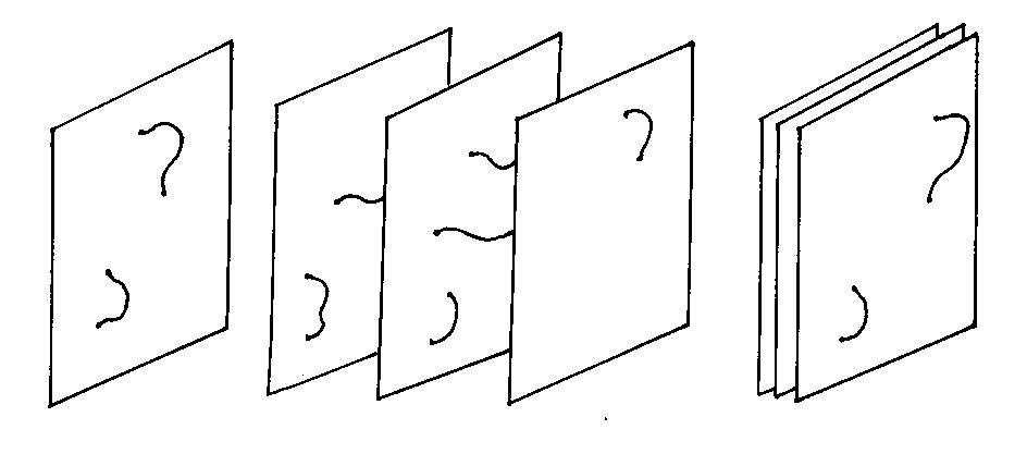
Open strings whose endpoints are attached to a single brane can have arbitrarily short length, and must therefore be massless. This excitation mode induces a massless U(1) gauge theory on the world brane, which is effectively 4-dimensional flat spacetime. Since the brane breaks half of the number of supersymmetries, it is ½ BPS. The U(1) gauge theory must have N = 4 Poincare supersymmetry. In the low energy approximation, which has at most two derivatives on bosons and one derivative on fermions, the N = 4 supersymmetric U(1) gauge theory is free.

With a number N > 1 of parallel separate D3-branes, the endpoints of the strings could be on different branes. There are N² – N such possible strings. In the limit where the N branes tend to be coincident, all string states would be massless, and the U(1)^N gauge symmetry is enhanced to a full U(N) gauge symmetry. Separating the branes is then interpreted as Higgsing the gauge theory to the Coulomb branch where the gauge symmetry is spontaneously broken.

The spacetime metric of N coincident D3-branes can be written as

ds² = (1 + L⁴/y⁴)^-1/2 n_ij dxⁱ dy^j + (1 + L⁴/y⁴) (dy² + y² d[omega]_s²)

where L is the radius of the D3-brane, and is given by

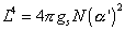
L⁴ = 4[pi]g_s N([alpha]’)²

There are two regimes to look at. As y >> L, you get flat spacetime R¹⁰. When y < L, you get the throat, and it becomes singular as y << L.

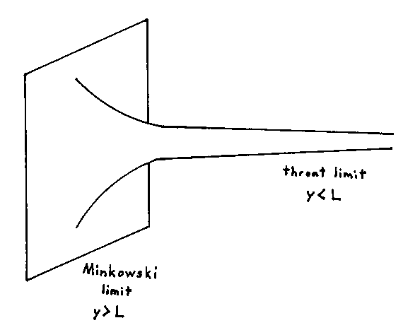
With the redefinition

u = L²/y

and in the large u limit, the metric becomes

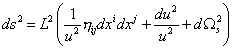
ds² = L² [1/u² n_ij dxⁱ dx^j + du²/u² + d[omega]_s²)

which corresponds to a product geometry. One component is the five-sphere S⁵ with the metric

L² d[omega]_s²

The remaining component is the hyperbolic space AdS₅ with the constant negative curvature metric.

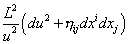
L²/u² (du² + n_ij dxⁱ dx_j)

Therefore, the geometry close to the brane, y = 0, or u = ∞, is regular and symmetrical, and may be summarized as AdS₅ x S⁵, where both components have identical radius L.

The Maldacena limit corresponds to keeping g_s and N fixed, as well as all physical length scales fixed, and letting α’ → 0. In the Maldacena limit, only the AdS₅ x S⁵ region of the D3-brane geometry survives the limit, and contributes to the string dynamics of physical processes, while the dynamics in the asymptotically flat region decouples from the theory.

The AdS/CFT or Maldacena conjecture states the equivalence or duality between the following two theories.

1. Type IIB superstring theory on AdS₅ x S⁵ where both AdS₅ and S⁵ have the same radius L, where the 5-form F_s⁺ has the integer flux

N = [integral over S⁵] F_s⁺

And where the string coupling is g_s.

2. N = 4 supersymmetric Yang-Mills theory in 4 dimensions, with gauge group SU(N) and Yang-Mills coupling g_YM in its superconformal phase.

with the following identifications between the parameters of both theories.

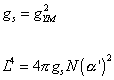
g_s = g_YM²

L⁴ = 4[pi]g_s N([alpha]’)²

And the axion expectation value equals the SYM instanton angle < C > = θ_I. Equivalence includes a precise map between the states and fields on the superstring side, and the local gauge invariance operators on the N = 4 SYM side, as well as a correspondence between the correlators of both theories.

The ‘t Hooft limit consists of keeping the ‘t Hooft coupling

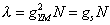
fixed, and letting N -> [infinity].

In Yang-Mills theory, this limit is well defined, at least in perturbation theory, and corresponds to a topological expansion of the field theory’s Feynman diagrams. On the AdS side, you can interpret the ‘t Hooft limit by saying that the string coupling constant can be expressed in terms of the ‘t Hooft coupling as

g_s = [lambda]/N

Since λ is being kept fixed, the ‘t Hooft limit corresponds to weak coupling string perturbation theory.

After taking the ‘t Hooft limit, where λ = g_s N is kept fixed while N → ∞, the only parameter left is λ. Quantum field theory corresponds to λ << 1. On the AdS side, it is natural to take λ >> 1 instead.

At the end of my paper on the Standard Model, I listed questions left unanswered by the Standard Model, and one of the questions was “Why is gravity so much weaker than the other forces?” Nothing that I’ve said so far addresses this question. However, this question is successfully addressed by a theory called the brane world scenario or brane world cosmology, the premise of which is that not all of the extra dimensions are compactified. Up until now, we have assumed that the reason we don’t detect the extra dimensions is because they are compactified on distance scales on the order of the Planck length. However, they would also not be detectable by us if all the fermions and gauge bosons were confined to a D3-brane within higher dimensional space. Remember, in Type I string theory, the fermions and gauge bosons are open strings, while the gravitons are closed strings. It’s easier to visualize with the following example. Let’s say that the open strings were all attached to a D2-brane, while the closed strings move freely throughout 3D space.

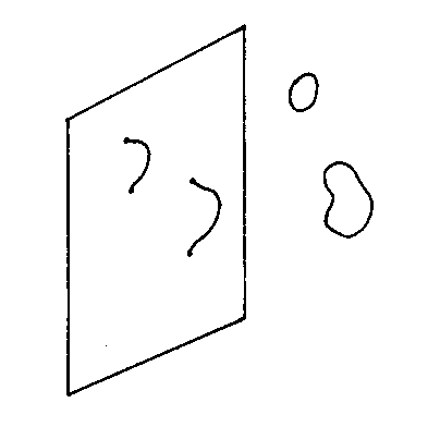
The fermions and gauge bosons, which are open strings, would be forced to slide around on a 2D plane, while the gravitons, which are closed strings, would have more room to move around, and would be floating around in 3D space. Therefore, the fermions and gauge bosons would interact with each other much more frequently than they would interact with the gravitons. Let’s say the fermions and gauge bosons were permanently attached to a D3-brane that is embedded within four spatial dimensions. From the point of view of the fermions and gauge bosons, the universe would appear to have three spatial dimensions, since they are confined to the D3-brane. However, the gravitons would have no such restriction, since they can move freely throughout the four spatial dimensions. You would then have an extra dimension which is not detectable by us even though it’s not compactified. Also, because the gravitons have the extra dimension to move around in, they would only rarely interact with the fermions and gauge bosons, which are stuck in three dimensions. The fermions and gauge bosons would interact with each other far more frequently than they would interact with the gravitons. Therefore, gravity would appear far weaker than the other forces. According to this theory, our entire Universe would be a giant D3-brane. Since, you’re assuming our world is a brane, this is called the brane world scenario or brane world cosmology. It assumes that our universe is a D3-brane, which has three spatial dimensions or four spacetime dimensions, and is embedded within a higher dimensional spacetime, which has four spatial dimensions or five spacetime dimensions. This higher dimensional spacetime is called the bulk, as opposed to our universe, which is called the brane. One version of the brane world scenario is called the Randall-Sundrum model, which assumes that our universe is one of two parallel D3-branes, and gravity originates on the other one.

The brane world scenario also provides an alternative explanation for the hierarchy problem. Quantum corrections to the Higgs mass would drive the Higgs mass up to the highest energy scale. If there were no physics beyond the Standard Model, it would only drive it up to the top quark mass, and there would be no problem. However, in grand unified theories, the Higgs mass would be driven up to the grand unification scale of 10¹⁶ GeV. More likely, there is some sort of theory of quantum gravity, and the Higgs mass would be driven up to the Planck scale of 10¹⁹ GeV. However, the Higgs mass cant be higher than about 1 TeV without violating unitarity. The most common explanation for this is supersymmetry. Above the supersymmetry breaking scale, fermionic and bosonic contributions to the Higgs mass would cancel out, leaving a Higgs mass of about 1 TeV. However, the brane world scenario provides a different solution to this problem. Gravity appears weak to us only because we are confined to the brane, and within the bulk, gravity is not as weak as it appears to us. Therefore, gravity is not really as weak as it appears. Therefore, the Planck scale is not really as high as it appears. The weaker gravity, the higher the Planck scale would be. The stronger gravity, the lower the Planck scale would be. Due to the running of the coupling constants, the coupling constants converge, but the farther they are apart, the longer it would take for them to converge. Gravity is so much weaker than the other forces, it would only have the same strength as the other forces if you go all the way up to the Planck scale. However, if gravity is not really that weak, then the Planck scale is not really that high. The quantum corrections to the Higgs mass would drive it up to the highest energy scale, but if the real Planck scale is much lower than it appears to us, then that’s the highest energy scale, and the Higgs mass would only be driven up to that. The Higgs mass would be much lower, and you can solve the hierarchy problem. Therefore, in addition to providing an interesting explanation to the otherwise unanswered question of why gravity is so weak, the brane world scenario also provides an alternative explanation for the hierarchy problem. One thing that’s confusing is that some people use the phrase “hierarchy problem” to refer specifically to the question “Why is gravity so much weaker than the other forces?” which is a related but different question than the usual meaning of the phrase, which is how do you keep the Higgs mass low enough as to not violate unitarity.

In Heterotic E₈ x E₈ superstring theory, you have 10-dimensional spacetime, with 9 spatial dimensions, bounded by two 9-dimensional spacetime boundaries, each with 8 spatial dimensions. You then compactify it on a Calabi-Yau manifold, which has 6 dimensions, leaving 4-dimensional spacetime, with 3 spatial dimensions, bounded by two 3-dimensional spacetime boundaries, each with 2 spatial dimensions. In M-theory, there are 11 spacetime dimensions. Heterotic E₈ x E₈ superstring theory inspired Heterotic M-theory. You have 11-dimensional spacetime, with 10 spatial dimensions, bounded by two 10-dimensional spacetime boundaries, each with 9 spatial dimensions. You then compactify it on a Calabi-Yau manifold, which has 6 dimensions, leaving 5-dimensional spacetime, with 4 spatial dimensions, bounded by two 4-dimensional spacetime boundaries, each with 3 spatial dimensions. One of these can then be identified with our Universe, according to the brane world scenario. The more common way to compactify M-theory is to take 11-dimensional spacetime, with 10 spatial dimensions, and compactify it on a Joyce manifold, which has 7 dimensions, leaving 4-dimensional spacetime, with 3 spatial dimensions.

Fundamental particles are superstrings, which are D1-branes, and the Universe is a D3-brane. Therefore, “fundamental particle” and “Universe” are just different subcategories of the same type of thing, which are D-branes. There could be many D3-branes, each of which you could call a different universe, and they could act like fundamental particles. A D3-brane, and anti-D3-brane could be created from the vacuum, and then annihilate each other, analogous to an electron and positron being created from the vacuum, and then annihilating each other. A D3-brane and anti-D3-brane could form a bound state called branonium, analogous to an electron and positron forming a bound state called positronium. You have the unusual situation that our universe could be a fundamental particle in an atom in higher dimensional spacetime.

There is a long standing theory in cosmology that our universe has gone through an infinite number of cycles, where each Big Bang is preceded by a Big Crunch, and each Big Crunch is followed by a Big Bang. This is called cyclical cosmology, and it’s a small minority of cosmologists that ascribe to it. Brane world cosmology has inspired a version of cyclical cosmology, in which our universe is one of two parallel D-branes which are attracted to each other. When they impact, they bounce apart, and this is experienced as a Big Crunch/Big Bang on the D-branes. After they recoil, they are attracted to each other, and the process starts again. The main problem with this theory is that it has to pass through a singularity at each collision. The problem of the singularities is an endemic problem in all theories of cyclical cosmology.

Most cosmologists instead ascribe to inflationary cosmology. The original Big Bang model suffered from the flatness problem, the horizon problem, and the monopole problem. How can the Universe be as flat as the isotropy of the cosmic microwave background would seem to indicate? How can distant parts of the Universe that aren’t casually connected be so similar? Why haven’t we detected magnetic monopoles? All of these problems are solved by inflationary cosmology, which is assuming that the Universe went through a period of enormous inflation shortly after the Big Bang. During an internal of time on the order of the Planck time, a sphere with a radius of the Planck length would expand to several orders of magnitude larger than the current observable Universe. In conventional slow roll inflation, the Universe undergoes an expansion of a least 10²⁶ during the inflationary phase. Such rapid expansion would flatten the Universe. Regions that were originally very close would become very distant but still remain similar. It’s very unlikely that any monopoles would end up in our observable Universe. Inflationary cosmology solves the flatness, horizon, and monopole problems. There is also experimental evidence for inflationary cosmology. The details of the cosmic microwave background as determined from COBE, Boomerang, Maxima, and most recently WMAP, provide overwhelming evidence for inflationary cosmology. The WMAP probe mapped the anisotropy of the cosmic microwave background to extraordinary precision, and the angular power spectrum of the temperature fluctuations in the cosmic microwave background were a very close match to the prediction from inflationary cosmology. In addition, from studying supernovae Ia, we can tell that the expansion of the Universe is accelerating, although obviously much less than it was originally. This all implies an effective positive cosmological constant, or some variation, such as quintessence, which is a rolling scalar field. This in turn requires de Sitter space, or something similar to it. De Sitter space can be defined as the maximally symmetric space with positive cosmological constant.

Empty de Sitter space is the unique spacetime with maximal symmetry and constant positive curvature. In D spacetime dimensions, it is locally characterized by

R_ab = ((D – 1)/R²) g_ab

where R is the radius of curvature of de Sitter space, and by the vanishing of the Weyl tensor. The cosmological constant Λ is a function of R. With the local geometry fixed, the only remaining freedom is the global topology. You can think of de Sitter space as a timelike hyperboloid embedded in (D-1)-dimensional Minkowski space. The embedding equation is

-X₀² + X₁² + …+X_D² = R²

where X_I are Cartesian coordinates in Minkowski space. This makes the O(1, D) isometry group of de Sitter space obvious. O(1, D), the Lorentz group in D + 1 spacetime dimensions, has four disconnected components. These are the proper orthochronous Lorentz group, and its composition with the discrete symmetries P and T.

In de Sitter space, there is a problem in defining the S-matrix. In quantum field theory, asymptotic incoming and outgoing particles are properly defined only in the asymptotic region of spacetime. However, for de Sitter space, these regions are spacelike, and there is no single observer who can determine the states both at past infinity and future infinity. Therefore, the S-matrix elements in de Sitter space are not measurable quantities. They are metaobservables instead of observables. When you take into account quantum gravity in asymptotically de Sitter space, the problem becomes more severe. Witten pointed out that the only available pairing between in states and out states, CPT, is used to obtain an inner product for the Hilbert space. There does not seem to be an additional pairing between in and out states that could be used to arrive at an S-matrix. Since the conventional formulation of string theory is based on the existence of an S-matrix, this was a serious problem in trying to reconcile string theory with inflationary cosmology.

One attempt to make superstring theory consistent with inflationary cosmology was called pre-Big-Bang cosmology, which was based on trying to use the scalar fields already present in superstring theory to drive the inflation. This was only moderately successful. Another idea was to try to obtain de Sitter space from supergravity by reducing it on non-compact internal spaces, or by supergravity with negative norms. However, despite such valiant efforts, this appeared in to be such an intractable problem, that physicists talked about no-go theorems that supposedly proved that de Sitter space can’t be embedded into 11-dimensional supergravity.

It is therefore a great achievement, not to mention a relief, that recently, we have been able to expand M-theory to allow for de Sitter space. This is a very important result because we are finally unifying M-theory with inflationary cosmology. What you basically do is expand the moduli space of M-theory to include points that allow for de Sitter space. An example of this expanded M-theory is called MM-theory, developed by A. Chamblin and N. D. Lambert in 2002. Instead of using the standard spin connection D, they used a conformal spin connection

[D hat] ~ D + 2k

provided that the conformal part of the curvature vanishes. dk = 0 In simply connected spacetimes, this implies that k is exact, and the modification is simply a field redefinition. If k = dθ, then the redefinition that takes the equations of motion defined with the connection [D hat] back to the usual ones

e_M^N -> e^-2[theta] e_M^N

[psi]_u -> e^-2[theta] [psi]_u

where M, N = 0, 1,1…0. However, if the spacetime is non-simply connected, then this modification is non-trivial.

Let’s compactify M-theory on M₁₀ x S¹. You can then choose k = m dy, where dy is the tangent vector to the circle. If you turn off the four-form field strength and the fermions, then the equations of motion of the compactified theory in 10 dimensions are

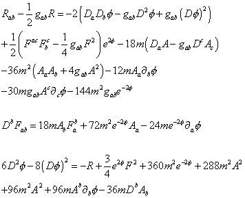
R_ab – ½g_ab R = -2(D_a D_b [phi] – g_ab D² [phi] + g_ab + g_ab (D[phi])²) + ½ (F^ac F_b^c – ¼ g_ab F²) e^2[phi] – 18m(D_a A_b – g_ab D^c A_c) – 36 m² (A_a A_b + 4 g_ab A²) – 12 m A_a[partial derivative]_b [phi] – 30mg_ab A^c [partial derivative]_c [phi] – 144m² g_ab e^-2[phi]

D^b F_ab = 18m A_bF_a^b + 72 m²e^-2[phi]A_a -24me^-2[phi] [partial derivative]_a [phi]

6D² [phi] – 8(D[phi])² = -R + ¾ e^2[phi] F² + 360m² e^-2[phi] + 288m² A² + 96m² A² + 96mA^b [partial derivative]_b [phi] – 36mD^b A_b

If you turn off all the gauge potentials, you are left with Einstein equation

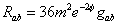
R_ab = 36m² e^-2[phi] g_ab

Together with the Maxwell and scalar equations which imply that the dilaton φ is a constant. Therefore, if you turn off all of the fields except gravity, you get 10-dimensional de Sitter space. The effective cosmological constant is

[capital lambda] = 576 m² e^-2[phi]

It now appears that within the entire moduli space of M-theory, or perhaps an expanded version of M-theory, there are points that allow for de Sitter space. M-theory then allows for inflationary cosmology. You could even say that we have achieved unification between the most advanced theoretical particle physics and cosmology. In inflationary cosmology, there are an infinite number of tiny regions of the early Universe that expanded to be larger than the observable Universe today. Since they are no longer casually connected, you could think of them as different universes. In eternal inflation, this has been going on for an infinite length of time. There are then an infinite number of universes, each of which corresponds to a different point in the moduli space of M-theory, and therefore, end up with different forces, particles, etc. The one we are in would then be selected using the anthropic principle. This seems to be a basically self-consistent description of the Universe that encompasses all of physics, and is the majority view among physicists. This is currently our basic view of the Universe.

However, Leonard Susskind gave a talk at a cosmology conference in Davis in March 2003, where he explained why we should temper our enthusiasm. It’s very probable that there is some point in the moduli space of M-theory that corresponds to the real Universe, but very unlikely that we will ever identify it. There are an infinite number of points in the moduli space of M-theory. There are thousands of free parameters, such as the precise details of the topology, the compactification, the wrapping modes of branes, fluxes, etc. Susskind called this vast parameter space encompassing all the possible values of all the possible free parameters, the landscape. Susskind estimates there are 10⁵⁰⁰ string vacua. It’s very unlikely that we’ll ever identify the precise point in the infinite moduli space of M-theory that corresponds to the real Universe. We don’t know which point it is, but we know which points it’s not, namely it’s none of the points we know about. Specifically, none of the five superstring theories which we’ve studied so exhaustively correspond to the real Universe since they don’t allow for de Sitter space. Therefore, at least for the foreseeable future, it looks like we’ll have to give up on the longstanding hope of using superstring theory or M-theory to actually calculate the parameters of the Standard Model or extensions of the Standard Model, much less shed new light on quantum gravity.

It appears that the octonions are relevant to M-theory. Therefore, to understand M-theory at a deeper level, you should study the octonions. For an excellent review of the octonions, read John Baez’s paper “The Octonions”.The Octonians

A division algebra is an algebra for which if ab = 0, then either a = 0, b = 0, or a = b = 0. There are four normed division algebras which are the real numbers, complex numbers, quaternions, and octonions.

The real numbers R are a one-dimensional algebra that can be placed in order.

a

The complex numbers C are a two-dimensional algebra that have no order but are commutative and associative.

a + bi

where i² = -1

The quaternions H are a four-dimensional algebra that are not commutative but are associative.

a + bi + cj + dk

where i² = j² = k² = ijk = -1

In other words, the quaternions H are a four-dimensional algebra with basis 1, i, j, k where

1 is the multiplicative identity

i, j, k are the squareroot of -1

ij = k, ji = -k, and all identities obtained from these by cyclic permutations of (i, j, k)

Quaternions were invented by William Rowan Hamilton in 1843.

The octonions O are an eight-dimensional algebra that are not associative but are alternative, which is a weaker form of associativity. The octonions O are an eight-dimensional algebra with basis 1, e₁, e₂,…e₇ where

1 is the multiplicative identity

e₁, e₂,…e₇ are the squareroot of -1

Their multiplicative rules are summed up by a diagram called the Fano plane. If you multiply two numbers on a line, their product is the third number on that line. If you have to go in the opposite direction as the arrows, you add a minus sign to he next number on the line.

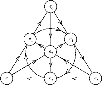
Octonians were invented by John T. Graves in 1844. For more information on octonions, read John Baez’s paper. M-theory displays geometric and algebraic structures derived from the octonions. The octonions are related to the exceptional Lie groups, G₂, F₄, E₆, E₇, and E₈. Compact manifolds of G₂ holonomy called Joyce manifolds, discovered in 1996, play a fundamental role in compactifying M-theory. The four coincidences in the list of simple Lie groups are

A₁ = B₁ = C₁

SU(2) = Spin(3) = Sp(1)

B₂ = C₂

Spin(5) = Sp(2)

A₃ = D₃

SU(4) = Spin(6)

D₂ = A₁ x A₁

Spin(4) = SU(2) x SU(2)

Are related to some irreducible representations of the exceptional Lie groups. They also appear in physics such as compactifications of M-theory disguised in various forms.

The four lists of classical supersymmetric p-branes, including instantons, embedded in D-dimensional spacetime correspond to the four normed division algebras R, C, H, and O.

Real ladder: From D = 1, p = -1 instanton (kink) to D = 4, p = 2 membrane (domain wall, codimension one)

Complex ladder: From D = 2, p = -1 instanton (vortex) to D = 6, p = 3 universe (codimension two)

Quaternionic ladder: From D = 4, p = -1 instanton to D = 10, p = 5 5-brane (codimension four)

Octonionic ladder: From D = 8, p = -1 Fubini-Nicola instanton to D = 11, p = 2 M2-brane

These four ladders can be thought of as oxidation of the corresponding instanton in its turn associated to the fundamental line bundle for the projective spaces KP¹, where K = R, C, H, and O. The four are supersymmetrizable, and are linked as the four Hopf bundles. The Cayley plane OP² is related to the 11d supergravity corner of M-theory.

Compactifying 11d supergravity from the original 11d to 4d causes all of the E series split forms to appear successively. The moduli spaces of scalar fields are homogenous spaces. The Heterotic E₈ x E₈ superstring theory makes direct use of E₈ x E₈. Also E₆ appears in the compactification of E₈ x E₈.

In 10d superstring theory, it was common to compactify the extra dimensions on Ricci-flat Calabi-Yau manifolds. In 11d M-theory, it’s common to compactify the extra dimensions on G₂-manifolds called Joyce manifolds, discovered in 1996. G₂ compact holonomy manifolds are still Ricci-flat, and conserve 32/4 = 4 supercharges, which gives N = 1 supersymmetry in 4 dimensions. From the reduction of the tangent bundle of a compactifying space K₇, you get

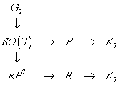
G₂ holonomy involves some torsion properties in K₇. The reason for the descent SO(7) to G₂ is because the later conserves a 3-form related to the octonionic product, and probably related to the 3-form in M-theory in the 11d supergravity limit.

In 1914, Elie Cartan noticed that the smallest of the exceptional Lie groups, G₂, is the automorphism group of the octonions. Its Lie algebra g₂ is therefore der(O), the derivation of the octonions. G₂ is the subgroup of Spin(7) fixing the unit vector in S₇. Since Spin(7) acts trivially on the unit sphere S⁷ in this spinor representation, you have

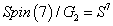
Spin(7)/G₂ = S⁷

Both Im(H) and Im(O) are equipped with a 3-form, or an alternating trilinear function, given by

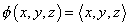
[phi](x, y, z) = x, y, z

In the case of Im(H), this is just the usual volume form, and the group of real linear transformations preserving it is SL(3, R). In the case of Im(O), the real linear transformation preserving φ are those in the group G₂. The 3-form φ is important in Joyce manifolds, which are 7-dimensional Riemannian manifolds with holonomy group equal to G₂.

The following equation is actually a pun.

F = MA_{T² -> 0}

This proves that M-theorists have a sense of humor, albeit an esoteric one, as can be expected. This is the Aspinwall-Schwarz equation which describes how a general compactification of F-theory arises from M-theory. M-theory is compactified on an elliptically fibered manifold X, and the area of the fibers is then scaled to zero. However, any physics student who sees the above equation would be instantly reminded of Newton’s Second Law, F = ma, which is probably the second most famous equation in physics, second only to E = mc². Perhaps one person out of a hundred would recognize Newton’s Second Law, but only one physicist out of a thousand would recognize the Aspinwall-Schwarz equation, so this is very much an inside joke.

D-branes have been used to calculate the entropy of black holes. Strominger and Vafa have shown that D-brane techniques can be used to count the quantum microstates associated with classical black hole configurations. The simplest case, which was studied first, is static extremal black holes in five dimensions. Strominger and Vafa showed that for large values of the charges, the entropy, defined by S = log N, where N is the number of quantum microstates that the system can be in, agrees with the Bekenstein-Hawking prediction of ¼of the area of the event horizon. This result has been generalized to black holes that are near extremal and radiate correctly, or rotating.

D-branes are surfaces on which open strings can end. Their dynamics are described by open string theory, as described by Witten. However, this can be difficult to work with in practice, so it is sometimes useful to consider the low energy effective action obtained by integrating out all the massive modes, keeping only the massless super-Maxwell multiplet. This becomes practical only if you keep terms in which the fields are slowly varying at the string scale, keeping the field strengths but not their derivatives. The field strengths are allowed to be large but they can’t exceed a certain critical value. At this value, the stretching force on a string with charges on its ends matches the string tension. In the case of Type II superstrings, the effective action is the sum of two terms, a Dirac-Born-Infeld term and a Chern-Simons term.

S = S_DBI + S_CS

The following versions of superstring theory are the most successful in terms of reproducing the particle spectrum from the Standard Model.

1. The most conventional one is E₈ x E₈ Heterotic superstring theory which was invented in 1985 by Gross, Rohm, Harvey, and Martinec. It has 10 spacetime dimensions, six of which are compactified on a six-dimensional Calabi-Yau space ,also called Calabi-Yau three-fold, where 3 is the complex dimension. This realistic compactification was discovered by Strominger, Witten, Candelas, and Horowitz. In the realistic models, one of the E₈ gauge groups is broken to E₆ to SO(10) to SU(5), which is subsequently broken to the Standard Model’s SU(3) x SU(2) x U(1). Usually we are looking for the N=1 supersymmetric extensions of these theories, assuming that SUSY is broken spontaneously. You get the correct spectrum of gauge bosons as well as fermions, with the right-handed neutrino included, and some extra fermions that complete the 27 representation of E₆. You can also calculate the number of generations, which you can arrange to be three.

2. If the model above has a coupling constant that is stabilized around a large value, a new 11th dimension of M-theory emerges. Because you started with the Heterotic theory, the new 11th dimension will have two boundaries, each of them carrying a single gauge group E₈, which was found by Horava and Witten. The theory is called Heterotic M-theory or Horava-Witten theory. This extra 11th dimension can be in fact much larger than the 6 dimensions of the Calabi-Yau space, and therefore the world would appear as five-dimensional.

3. M-theory, the 11-dimensional theory, can also be directly compactified on 7-dimensional manifolds. They must have a G₂ holonomy to get N=1 supersymmetry in four dimensions, and they must contain a singularity if we want to reproduce the spectrum of chiral fermions. Interesting calculations in these models exist, such as proton decay, and this model is in some sense the most geometrical one, because all the extra stringy degrees of freedom beyond the visible 4 dimensions are treated geometrically.

4. F-theory, invented by Cumrun Vafa in 1995, is formally a 12-dimensional theory, but you must always compactify two of its dimensions on a two-torus, which effectively leads to type IIB string theory. F-theory on a (d + 2)-dimensional manifold M is a fancy way to describe a compactification of Type IIB strings on a d-dimensional manifold which is the base of the (d + 2)-dimensional manifold M. The fiber must be a two-torus. The shape of the two-torus determines the complex coupling constant of type IIB string theory. F-theory on eliptically fibered, where the fiber is a two-torus, Calabi-Yau four-folds, which are eight-dimensional, is a realistic theory because it leads to N=1 supersymmetry in four dimensions. Randall-Sundrum models have been constructed using these models.

5. Intersecting brane models often construct non-supersymmetric Standard Models with essentially the right spectrum. These particles are vibrating strings whose two ends are attached to different D-branes that intersect. Various particles are therefore forced to be localized at different intersections. These models can again be realistic, and they naturally lead to hierarchy of fermionic masses.

Fluxes are generalizations of the magnetic flux, and are being added to the previous models, and it leads to new useful physical features.

I have described superstring theory which is our main way of trying to quantize gravity. However, there do exist alternative theories of quantum gravity, at least one of which is worthy of mention, called loop quantum gravity. This is a radically different way of trying to approach the problem of a quantum theory of gravity. It actually has nothing to do with particle physics, and is instead derived from general relativity. Particle physicists view general relativity in the same way they do Newtonian mechanics. We use classical Newtonian mechanics all the time to solve practical problems, and for most purposes, it’s sufficient, but it’s obviously not true since it does not take into account relativity or quantum mechanics. Fermi’s theory of the weak force is adequate for many applications, although it’s obviously not true since it’s non-renormalizable and has no mediating particle, and is only a sufficient approximation in the low energy limit. Particle physicists view general relativity in the same way. They consider it a useful tool that we use all the time, but to them, it’s obviously untrue at a fundamental level. First of all, it doesn’t include quantum mechanics. Second of all, it describes gravity in a radically different way from the other forces, and from what particle physicists are used to. In particle physics, the four forces are caused by the exchange of virtual bosons, which in the case of gravity is the graviton. In general relativity, gravity is the curvature of spacetime itself. In general relativity, there is no such thing as a graviton. This is a fundamentally different way of thinking about gravity. According to general relativity, what we call gravity is actually the curvature of spacetime.

There are far more particle physicists then general relativists, so the particle physics view is the majority view. However, general relativists do exist, and these people take the general relativity view seriously. Even they admit that general relativity in the form Einstein invented can’t be true because it doesn’t include quantum mechanics. However, their solution is to come up with a quantum version of general relativity. They have had some success, and this quantum version of general relativity is called loop quantum gravity. It retains the general relativity assumption that gravity is literally the curvature of spacetime, instead of the exchange of a particle, so therefore quantizing gravity means you are somehow quantizing the curvature of spacetime. Normally, the curvature of spacetime is considered the background metric, except here, it’s the thing being quantized, so that means there is no background metric. This shows you what an unusual theory this is because this is probably the only field of physics where there is no background metric at all. This requires radically different mathematics than anything else in physics. From the point of view of loop quantum gravity theorists, the absence of a background metric is an additional benefit to the theory. They believe the real Universe doesn’t have a background metric, and so preferably, you should do physics without it. Loop quantum gravity makes absolutely no attempt to try to unify gravity with the other forces. Rather, what they are trying to unify is what they perceive to be the two fundamental theories left to be unified, which are general relativity and quantum mechanics.

Loop quantum gravity began in the middle of the 1980’s. The pioneers of the field include Amitaba Sen, Abhay Ashtekar, Ted Jacobson, Lee Smolin, and Carlo Rovelli. A more recent offshoot of loop quantum gravity is called spin foam theory. The mathematical tools for dealing with nonperturbative loop quantum gravity include Penrose’s spin network theory, SU(2) representation theory, Kauffman tangle theoretical recoupling theory, Temperley-Lieb algebras, Gelfand’s C* algebra spectral representation theory, infinite dimensional measure theory, and differential geometry over infinite dimensional spaces.

With loop quantum gravity, you start with classical general relativity, which can be formulated as follows. You fix a three-dimensional manifold M, and consider a smooth real SU(2) connection A_aⁱ (x) and vector density

[E tilda]_i^a (x) transforming in the vector representation of SU(2) on M, where a, b,…=1, 2, 3 for spatial indices, and i, j, …=1, 2, 3 for internal indices. The internal indices can be viewed as labeling a basis in the Lie algebra of SU(2), or in the three axis of a local triad. You indicate coordinates on M with x. The relation between these fields and conventional metric variables is as follows. [E tilda]_i^a (x) is the inverse triad related to the three-dimensional metric g_ab (x) of the constant time surfaces by

gg^ab = [E tilda]_i^a [E tilda]_i^b

where g is the determinant of g_ab and

A_aⁱ (x) = [capital gamma]_aⁱ (x) + [gamma] k_aⁱ (x)

where Γ_aⁱ (x) is the spin connection associated with the triad defined by

[partial derivative]_[ae_b]ⁱ = [capital gamma]_[aⁱ e_b]j

where e_a^j is the triad, k_aⁱ (x) is the extrinsic curvature of the constant time three surface.

γ is a constant called the Immirzi parameter. Different choices for γ give different versions of the formalism that are equivalent in the classical domain. If you choose γ to be equal to i.

[gamma] = [squareroot of –1]

then A is the standard Ashtekar connection, which can be shown to be the projection of the self-dual part of the four-dimensional spin connection on the constant time surface. If you choose γ = 1, you get the real Barbero connection. The Hamiltonian constraint of Lorentzian general relativity has a simple form in the

[gamma] = [squareroot of –1]

formalism. The Hamiltonian constraint of Euclidean general relativity has a simple form in the γ = 1 formalism. You can also choose other values of γ. It’s possible that quantum theory based on different choices of γ are inequivalent. There appears to be a unique choice of γ that gives the correct ¼ coefficient in the Bekenstein-Hawking formula.

The spinor version of the Ashtekar variables is given in terms of the Pauli spin matrices σ_i, where i = 1, 2, 3, or the SU(2) generators

[tau]_i = -i/2[sigma]_i

by

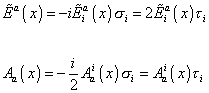
[E tilda] (x) = -i[E tilda]_i^a (x) [sigma]_i = 2[E tilda]_i^a (x) [tau]_i

A_a (x) = -i/2 A_aⁱ (x) [sigma]_i = A_aⁱ (x) [tau]_i

Thus A_a (x) and [E tilda]^a (x) are 2 x 2 anti-hermitian complex matrices.

The theory is invariant under local SU(2) gauge transformations, three-dimensional diffeomorphisms of the manifold on which fields are defined, as well as under coordinate time translations generated by the Hamiltonian constraint. The full dynamical content of general relativity is captured by the three constraints that generate these gauge invariances.

The Lorentzian Hamiltonian does not have a simple form if you use the real connection. For a long time, this was considered problem in terms of using the real connection to define the quantum Hamiltonian constraint. Therefore, they used the imaginary constraint. However, Thiemann figured out how to construct a Lorentzian quantum Hamiltonian constraint, despite the non-polynomiality of the classical expression. Therefore, today, the real connection is widely used. This has the advantage of eliminating the old reality conditions problem, which was the problem of implementing non-trivial reality conditions in the quantum theory.

You use the trace of the holonomy of the connection, which is labeled by loops on the three manifold, and higher order loop variables, obtained by inserting the E field, in n distinct points, into the holonomy trace. Given a loop a in M, with points s₁, s₂,…s_n in a, you have

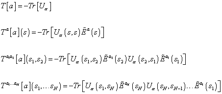
T[a] = -Tr[U_[alpha]

T^a[a] (s) = -Tr[U_[alpha] (s, s) [E tilda]^a (s)]

T^a₁a₂[a] (s₁, s₂) = -Tr[U_[alpha] (s₁, s₂) [E tilda]^a₂ (s₂) U_[alpha] (s₂, s₁) [E tilda]^a₁ (s₁)]

T^{a₁…a_N}[a] (s₁, …s_N) = -Tr[U_[alpha] (s₁, s_N) [E tilda]^a₂ (s_N) U_[alpha] (s_N, s_{N – 1})… [E tilda]^a₁ (s₁)]

where

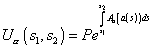
U_[alpha] (s₁, s₂) = Pe^{[integral from s₁ to s₂] A_a (a(s))ds}

in the parallel propagator of A_a along a defined by

d/ds U_[alpha] (1, s) = (da_a (s))/ds A_a (a(s)) U_[alpha] (1, s)

These are called the loop observables. The loop observables coordinatize the phase space, and have a closed Poisson algebra, denoted by the loop algebra. The Poisson bracket between

T[a] and T^c[beta] (s)

Is non-vanishing only if β (s) lies over a. If it does, the result is proportional to the holonomy of the Wilson loops obtained by joining a and β and their intersection.

{T[a], T^a[beta] (s)} = [triangle]^a [a, [beta] (s)] [T[a # [beta]] – T[a # [beta]^-1]

where

[triangle]^a [a, x] = [integral] ds (da^a (s))/ds [delta]³ (a(s), x)

is a vector distribution with support on a, and a # β is the loop obtained starting at the intersection between a and β, and following first a and then β. β^-1 is β with reversed direction.

A non-SU(2) gauge invariant quantity that plays a role in certain aspects of the theory, such as in the regularization of certain operators, is obtained by integrating the E field over a two-dimensional surface S

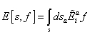
E[S, f] = [integral over S] dS_a [E tilda]_i^a f

Where f is a function on the surface of S, taking values in the Lie algebra of SU(2). Instead of loop observables, you could also take the holonomies and E[S, f] as elementary variables, which is more natural in the C*-algebraic approach.

There are probably ten times as many string theorists as loop quantum gravity theorists. Therefore, string theory is very much the majority view among physicists trying to quantize gravity. It’s very common for you to have two competing theories, and one becomes the majority view, and the other becomes an alternative view. Then the majority view becomes our view of the Universe, and the alternative view fades into memory. Sometimes, it’s because the majority view really is better at explaining what we observe or what we’ve been trying to explain. Sometimes, it’s not really better. Let’s say you have two theories. If someone just happens to think up a solution to one of the problems in one theory, people’s ears will perk up, and they’ll pay more attention to that theory. If there is a belief that one theory is more successful, that will cause more people to pursue that theory. More physics grad students will go into an exciting field that has had recent successes. It will attract more funding. Physicists hope that if it has had recent successes, that implies it will have more successes in the future. However, that becomes a self-fulfilling prophesy because obviously if more physicists are working on one theory instead of another theory, that will cause more progress in the theory with more physicists working on it. The more people trying to figure out how to solve the problems with a theory, the more likely someone will figure something out. You set up a positive feedback loop. The more people working on it, the more progress there will be, which will cause more people to work on it, etc. I don’t mean to say that’s the only thing that causes one theory to be chosen over another. Sometimes, one theory really is better than another. You just have to keep in mind that to some extent, it is a popularity contest. I think it’s good to have more than one theory since it reminds you that none of our theories are the real truth.

You can point to many examples where there is a main theory, that represents the majority view among physicists, and that becomes our view of the Universe, which has or had at least one serious rival, which was less popular, but was a serious alternative theory. The hadrons and the strong force were explained by QCD, although Regge theory was an alternative theory. The hierarchy problem was explained by supersymmetry, although technicolor was an alternative theory, and today the brane world scenario provides an alternative explanation. Quantum gravity is mainly explained by superstring theory, although loop quantum gravity is a serious alternative theory. The rotations of galaxies is explained by dark matter, although MOND was an alternative theory. Most cosmological data, such as the cosmic microwave background, is explained by inflationary cosmology, although the cyclical model is an alternative to inflation.

It’s more complicated than just one theory beating out another, since physicists draw inspiration from anything they can, even theories that have been ruled out. Remember that string theory had its origin in Regge theory which we now consider a totally defunct historical theory. Doubtlessly, loop quantum gravity will have some influence on our view of the Universe. However, I think we can safely say that our view of the Universe in the future will be mainly derived from superstring theory and M-theory.

Lastly, there is one curious thing which may or may not be important. Even though superstring theory and loop quantum gravity approach the problem of quantizing gravity from totally different directions, and involve radically different mathematics, they both require the existence of some sort of circular structure. For superstring theory, it is the closed strings. For loop quantum gravity, it is loops. This possibly might be telling us something about the real Universe.