physics613

Cosmology is the study of the entire Universe on the grand scale. Therefore, the two most important subjects in existence are cosmology and particle physics, since they attempt to explain the Universe on the grand scale and the most fundamental scale. These two fields are intimately connected. Even though cosmology is one the most important human endeavors, many physicists feel that it has only recently become a serious science in the sense of being testable. Some cosmologists have heralded a new golden area of precision cosmology. We have recently obtained a wealth of new cosmological data from probes and other experiments designed to measure anisotropies of the cosmic microwave background or CMB, especially from the Wilkinson Microwave Anisotropy Probe, or WMAP. We can now say with certainly that the Big Bang occurred 13.7 ± 0.2 billion years ago, and the cosmic microwave background is a snapshot of the Universe 379 ± 8 thousand years later, when atomic nuclei and electrons first combined into atoms, thus becoming transparent to photons. We also have important recent data measuring the redshifts of distant Type Ia supernovae, which establish that the Universe is about 70% dark energy, and 30% matter, 98% of which is dark matter. In other words, Ω_Λ = 0.7, Ω_m = 0.3, and Ω_Λ + Ω_m = 1, giving a spatially flat universe. The current cosmological data from a wide variety of sources, such as WMAP, other CMB observations, Type Ia supernovae redshifts, the Lyman alpha forest, primordial deuterium abundances, and gravitational lensing are all consistent with each other as well as being consistent with the theoretical predictions of inflationary cosmology, which has been the predominate theory of cosmology since 1981. This is a great vindication to cosmology, not to mention a relief to cosmologists. In this paper, I use “Universe” with a capital U to mean the real Universe, and “universe” with a lower case u to mean a model universe. It would help if you have read my previous papers on Tensors, Lagrangians, The Standard Model, and Beyond The Standard Model.

The most primitive humans, which were nomadic tribes of hunter-gatherers, assumed the Universe was what they could personally see, which was the land stretching out to the horizon, forming a flat circular disk, with the sky above, forming a hemispherical dome. However, thousands of years ago, they had reason to think the Earth is round because when you see a ship go over the horizon, its sails are the last to disappear, and if you’re on a ship looking back at the land, the mountains disappear last. In the 6th Century B.C., the Pythagoreans, followers of Pythagoras of Samos (569 B.C. – 475 B.C.), claimed not just that the Earth was spherical, but that the Earth revolved around the Sun, or actually a “central fire” different from the Sun. Eudoxus of Cnidus (410 B.C. – 355 B.C.) attempted to explain the motion of the planets by using 27 spheres, and Callipus (370 B.C. – 300 B.C.) claimed that 34 spheres were needed. Aristarchus of Samos (310 B.C. – 230 B.C.) was an advocate of heliocentric motion. However, this view was a minority view, and most scientists believed in the geocentric system, such as that proposed by Claudius Ptolemy (85 A.D. – 165 A.D.). In order to explain the motions of the planets, they were assumed to periodically loop back upon themselves in epicycles. Archytas of Tarentum (428 B.C. – 350 B.C.) came up with an argument as to why the Universe was infinite, although most people assumed the Universe was finite, and was contained within the celestial sphere on which the stars were printed. The Ptolemaic system remained unchallenged until Nicholas Copernicus (1473 – 1543) in the 16th Century. Copernicus’ system did not match the accuracy of Ptolemy’s geocentric system. The reason was that Copernicus still assumed that the planets moved in circular orbits. This problem was solved when Johannes Kepler (1571 – 1630) proposed that they moved in elliptical orbits. Kepler proposed Kepler’s Laws. Kepler’s employer Tycho Brahe (1546 – 1601), who had a gold nose, advocated a system where the Sun and Moon orbit the Earth but the other planets orbit the Sun. Tycho also saw a supernova suggesting the heavens aren’t unchanging. When Galileo Galilei (1564 – 1642) turned the telescope to the sky, it revolutionized astronomy. He discovered moons of Jupiter, proving that not everything orbited the Earth. Due to Galileo, heliocentric motion became the majority view, yet even with the telescope, the stars looked the same, tiny pin pricks, of light, and he couldn’t detect any parallax, suggesting they were farther away than anyone imagined. Up until that point, it was assumed that the Solar System was the Universe. Then in the 1570’s, there was a shift, and it came to be believed that there was no celestial sphere, and the stars were scattered throughout space, which was the theory proposed by English astronomer Thomas Diggs in 1576. Isaac Newton (1643 – 1727) revolutionized physics with Newtonian mechanics which unified terrestrial and celestial mechanics. Pierre-Simon Laplace (1749 – 1827) mathematically explained all the dynamics of the Solar System. In 1823, Heinrich Olbers (1758 – 1840) put forward Olber’s paradox, which had been suggested by numerous people beforehand including Johannes Kepler, Edmund Halley, and Jean-Phillipe de Cheseaux, which was that there is an apparent paradox with an infinite universe, which is that we should see stars everywhere in the sky, but this was on the assumption that the Universe had existed for an infinite length of time. The first stellar parallax, which was of the star 61 Cygni, was measured in 1838 by Friedrich Wilhelm Bessel (1784 – 1846), who is better known for the Bessel functions. The nearest star turned out to be 25 trillion miles away. Parallax is like if you extend your arm, and stick out your thumb, and close one eye, and then close only the other eye, its apparent position against the background changes.

Since ancient times, it was recognized that most stars are in a bright band across the sky called the Milky Way, thought to resemble milk from the breast of the Greek goddess Hera. By the turn of the century, the Milky Way was recognized to be a giant disk shaped structure that contains most stars. However, most astronomers in the early 20th Century assumed that the Milky Way Galaxy was the Universe. Just as before, it was assumed that the Solar System was the Universe, it was now assumed that the Milky Way Galaxy was the Universe. There were a minority of people who disagreed with this. In 1755, philosopher Immanuel Kant (1724 – 1804) theorized that some of the nebula which astronomers saw might actually be galaxies like the Milky Way, very far away. Kant referred to them as “island universes”. In 1918, Shapley studied Cepheids, which are bright stars which pulsate at regular intervals from a few days to a month. Using Cepheid variables, he established that some of the nebula were very far away, proving the other galaxies theory. Starting in 1912, Vesto Slipher (1875 – 1969) measured spectra from the nebula, many of which are really galaxies, showing that many appeared to be Doppler-shifted. The Doppler effect is like when the pitch of the sound of a train seems to change as it goes pass you, although that’s not actually what’s happening with the galaxies. By 1924, Slipher had measured 41 nebulas, and 36 were red-shifted, meaning they were receding from us. This was made more rigorous by Edwin Hubble (1889 – 1953) in 1923 – 1929. Hubble was able to resolve Cepheids in the Andromeda galaxy using the 100-inch telescope on Mount Wilson. He developed a new distance measure using the brightest star for more distant galaxies. He correlated these measurements with Slipher’s nebula, and discovered Hubble’s Law, v = Hd, where v is the velocity, d is the distance, and H is Hubble’s constant, which he overestimated.

If all the galaxies were redshifted, that means they are all running away from each other, which means if you extrapolate backwards, the Universe must have had a beginning. Einstein would have been considered an even bigger genius than he was if he had predicted this ahead of time, which he could have since that’s what his own theory of general relativity suggested. You can’t really blame him for that since you think up theories to explain what you observe, and he thought up general relativity in 1915, and proposed a cosmological model in 1917, before there was much evidence that the Universe was expanding. Einstein inserted a term called the cosmological constant into his theory in order to allow for a static universe, which he later called the greatest blunder of his life. In 1917, Russian cosmologist Alexander Friedman (1888 – 1925) recognized that Einstein’s theory of general relativity allowed for an expanding universe. Einstein’s static universe was unstable. In 1917, Dutch astronomer William de Sitter (1872 – 1934) invented another static universe that turned out to be unstable, and then a universe that expands indefinitely was called a de Sitter universe. Model universes were studied by Russian cosmologist Alexander Friedman (1888 – 1925) in 1922 and 1924, and independently by Belgian priest Georges Lamaitre (1894 – 1966) in 1927. In 1930, Eddington proved that Einstein’s model was unstable, and proposed a non-static model. In 1933, A. G. Walker and H. P. Robertson independently proved that what we now call the Robertson-Lamaitre metric is the only one consistent with a homogenous isotropic universe. Despite the redshift data, many people denied that the Universe had a beginning. Fred Hoyle invented the name “Big Bang” as a derogatory insult of the theory that the Universe had a beginning, and the name stuck. Many people, including Fred Hoyle, Herman Bondi, and Thomas Gold, advocated the Steady State model, that the Universe had existed forever, and that new matter was constantly being created from nothing to fill in the gaps.

The great debate between the Big Bang theory and the Steady State theory was finally put to rest in favor of the Big Bang in 1964 when Arno Penzias and Robert Wilson discovered the cosmic microwave background radiation. Working with a 7.35 cm horn antenna at Bell Labs, Penzias and Wilson accidentally discovered an isotropic radio background. This cosmic microwave background was very strong evidence in favor of the Big Bang model, and it convinced most people. The temperature of this black body radiation is 2.725 K. This cosmic microwave background had actually been predicted by George Gamow in 1948, and by Ralph Alpher, and Robert Herman in 1949. Gamow had other advocates of the Big Bang had thought that all the elements had been created in the Big Bang. It turned out that only hydrogen and helium were produced in the Big Bang, and the other elements were created in stars. However, the relative abundances of the elements hydrogen and helium predicted by the Big Bang theory were in good agreement with observations. Despite these successes, there were problems with the Big Bang model, which were the horizon problem, the flatness problem, and the monopole problem. However, these problems are solved if you postulate an interval of enormous inflation in the very beginning of the Universe. This is called inflationary cosmology, and was originally invented by Starobinsky, and later developed by Alan Guth and Andrei Linde in 1981. Ironically, inflation, which saved the Big Bang model, raised the possibility of eternal inflation, which means the Universe could have existed for an infinite length of time after all. Also, in the 1970s, Rubin, Freeman, and Peebles measured the rotation curves of spiral galaxies, and found they did not obey Kepler’s Laws, specifically the velocity did not drop off with distance, which suggested the existence of dark matter. In 1986, de Lapparent, Geller, and Huchra did deep redshift galaxy surveys that demonstrated the existence of large scale structure in the form of huge bubbles, filaments, and sheets on scales from 25 megaparsecs to 100 megaparsecs. One parsec equals 3.09 x 10¹⁶ meters, or 3.26 light-years. In April 1992, the COBE satellite team announced the discovery of anisotropies in the cosmic microwave background at the level of one part in 100,000, proving how isotropic the Universe is. In 1995-1996, the Hubble telescope was able to resolve Cepheid variable stars in galaxies in the Virgo cluster, giving a much better calibration of the distance measures, and therefore a more accurate estimate of Hubble’s constant. In 1998, a balloon-based experiment called Boomerang in Antarctica measured the anisotropy of the cosmic microwave background. Also, in 1998, two separate teams, one led by Saul Perlmutter, and the other led by Brian Schmidt, announced their results from studying the redshifts from Type Ia supernovae, and determined that the expansion of the Universe is accelerating, so we do have some sort of effective cosmological constant after all. In June 2001, the WMAP probe was launched, and the results were published in February 2003, providing overwhelming confirmation of inflationary cosmology.

The general trend in the history of cosmology has been towards recognizing our own insignificance, for instance, that the Sun and other planets do not revolve around the Earth, our solar system is not the Universe, our galaxy is not the Universe, we are located on the edge of a typical galaxy that is only one of 100 billion galaxies in the observable universe, and baryonic matter, such as makes up us, constitutes only about two percent of all matter. This is called the Copernican principle, which states that we are typical observers, and there is nothing special about us. Rather than be disappointed by this blow to our ego, we should appreciate this fact which makes cosmology possible. If we are typical observers, we can be rest assured that our local region of space is representative of the Universe, and that observers anywhere in the Universe would see basically the same thing we see. Without that assumption, it would not be possible to do cosmology at all. However, there is also another principle called the anthropic principle that states that only certain parts of the Universe are likely to produce life, and so the mere fact we are here shows we are not in a completely typical part of the Universe. For instance, a point in the Universe chosen at random would be very unlikely to be as close to a star as we are. Of course, life could only arise near a star, which explains why we are close to a star.

The Copernican principle is related to two other concepts called homogeneity and isotropy. When Friedman, Robertson, and Walker tried to mathematically model the universe, they assumed it was homogeneous and isotropic because that was the simplest model, although they didn’t have evidence that it really was homogeneous and isotropic. Today, we know the Universe really is homogeneous and isotropic. Homogeneous means the universe is pretty much the same everywhere. Isotropic means that the universe looks the same no matter what direction you look. The diagram on the left is homogenous, and the diagram on the right is isotropic.

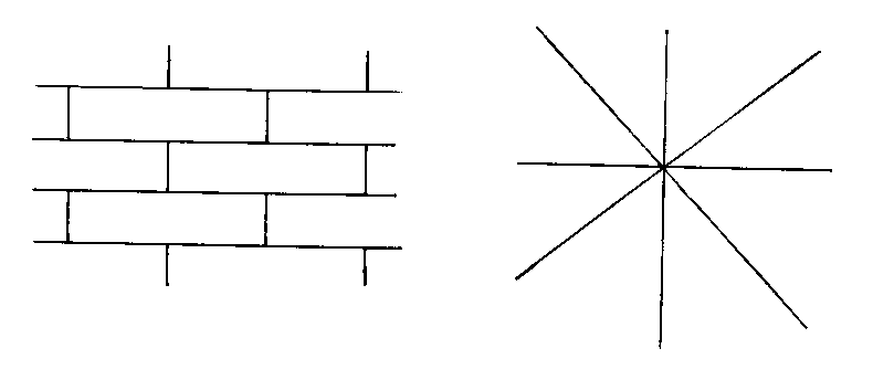
Another way of saying this is that homogeneous means it’s invariant under translations, and isotropic means it’s invariant under rotations. As another example, an infinite cylinder is homogenous but not isotropic. A cone is isotropic about the vertex but is not homogeneous.

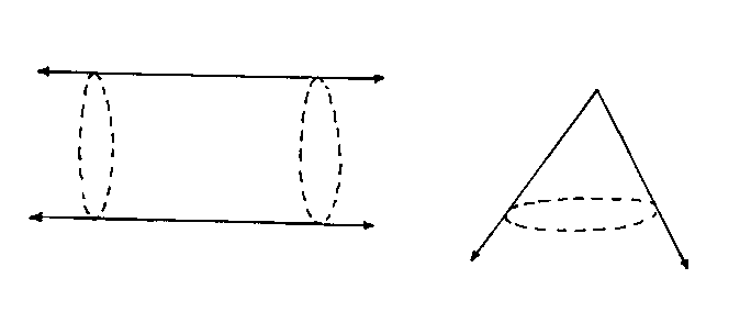
However, if the universe is isotropic about a single point, which it is for us, and you combine that with the Copernican principle, that requires the universe also be homogeneous. The Copernican principle states that if the universe is isotropic about one point, it is therefore isotropic about all points, and is therefore homogeneous. Imagine two intersecting circles.

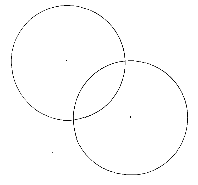
If the observer centered on one circle sees the same thing along the edge of his circle, then an observer centered on the other circle would see the same thing along the edge of his circle. The circles can be made of any size, so any observer would see the same thing everywhere, so the universe would be homogeneous. Therefore, isotropy plus the Copernican principle requires homogeneity. The reverse is not true. Homogeneity plus the Copernican principle does not require isotropy. However, we observe isotropy, and assume the Copernican principle, so we assume the Universe is both homogeneous and isotropic. The isotropy of the Universe is most obvious in the 2.725 K cosmic microwave background which is isotropic to one part in 10⁵.

In ancient Mesopotamia and Egypt, they had what we now call the Pythagorean theorem. The Egyptians used it to redraw the boundaries between farms after the annual flooding of the Nile. Pythagoras was one of the first ancient Greek scientists, although his followers formed a cult devoted to numerology. In the 6th century B.C., Pythagoras traveled to Egypt, learned of the Pythagorean theorem, and brought it back to Greece, where it was named after him. Today, it’s the mathematical concept named after the person who lived the longest length of time ago, and he didn’t even invent it. In the 19th Century, British schoolboys had to memorize the little ditty, “The area of the square on the hypotenuse is equal to the sum of areas of the squares on the other two sides.” This was also recited, inaccurately, by the Scarecrow in “The Wizard of Oz”. The quote from the Scarecrow was also repeated by Homer Simpson on “The Simpsons”. Let’s say you have two points on a Cartesian plane.

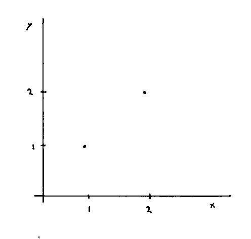
How would you find the distance between them? To find the distance between them, you subtract the x-coordinates and square the result, subtract the y-coordinates and square the result, add the results, and take the squareroot of that.

d = [squareroot of][(x₂ – x₁)² + (y₂ – y₁)²]

If you change the coordinate system, the calculated value for the distance between the points is the same.

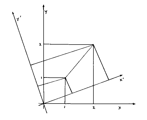
This means that the calculated distance between two points in invariant under a change of axes, which is exactly what you want in physics, since you don’t want the measured value of quantities to depend on your coordinate system. You see this concept of invariance throughout physics. You can rewrite the equation

d = [squareroot of][(x₂ – x₁)² + (y₂ – y₁)²]

as

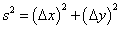
s² = (Δx)² + (Δy)²

which is the same under a change in axis.

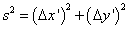
s² = (Δx’)² + (Δy’)²

You can also generalize it to three dimensions.

s² = (Δx)² + (Δy)² + (Δz)²

Now let’s look at spacetime according to classical Newtonian mechanics. Let’s say you have one time dimension, t, and two spatial dimensions, x and y.

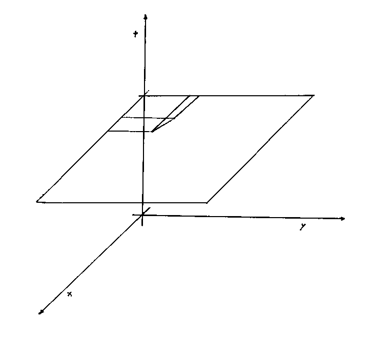
Now, in this system, you have an infinite number of horizontal x-y planes. Within each x-y plane, you can use the Pythagorean theorem to calculate the distance between two points, and the value is the same if you change the x and y axes, such as by rotating them around the t axis. So with an x-y plane at a given t coordinate, you can use the following formula

s² = (Δx)² + (Δy)²

However, the formula does not work for points that are not at the same t coordinate. In Newtonian mechanics, there is no way to calculate the distance between two points at different t coordinates.

You need some way of generalizing the Pythagorean theorem to allow for measuring the distance between two points with different t coordinates. Now in an x-y-z coordinate system, you would write

s² = (Δx)² + (Δy)² + (Δz)²

but you can’t do that on an x-y-t system because time obviously acts differently than the other dimensions. You need a way to convert between spatial dimensions and the time dimension. The conversion factor is the speed of light, where c = 2.99792458 x 10⁸ m/s. The correct formula for measuring the distance between points in the x-y-t system is

s² = -(cΔt)² + (Δx)² + (Δy)²

or in three spatial dimensions

s² = -(cΔt)² + (Δx)² + (Δy)² + (Δz)²

This is the coordinate system of special relativity. An event is specified by the coordinates (t, x, y, z), and the above defines the spacetime interval between two events. It can be positive, negative, or zero for non-identical points. The interval is unchanged by a change in coordinate system.

s² = -(cΔt’)² + (Δx’)² + (Δy’)² + (Δz’)²

This is called Lorentzian coordinates, whereas the x-y-z system is called Euclidean coordinates.

The coordinate transformations rotate space and time into each other. There is no fundamental concept of simultaneous events, since whether two events have the same t coordinate depends on the coordinate system used. So, here you have

s² = -(cΔt)² + (Δx)² + (Δy)² + (Δz)²

In order to simplify the notation, we frequently use naturalized units were c = 1, so then

s² = -(Δt)² + (Δx)² + (Δy)² + (Δz)²

Notice that if you replace t with t times i, you have (it)² and i² = -1, which cancels the minus sign in front of t, which turns the Lorentzian coordinates into Euclidean coordinates. This is called a Wick rotation.

In order to write the spacetime interval in more compact form, we introduce the following metric.

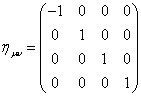
where sometimes it’s written with an opposite sign convention. So then, you have

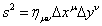
s² = n_uv Δx^uΔy^v

Before, in the Euclidean system, the distance between two points was the same if you did a translation or rotation of the axes. What kind of transformations leave the above spacetime interval unchanged? They include translations, rotations, and also boosts, which is going from a motionless frame of reference to one moving at a constant velocity. Boosts and rotations are called Lorentz transformations. Boosts, rotations, and translations are called Poincare transformations.

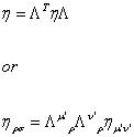
η = Λ^T η Λ

or

η_{ρ σ} = Λ^μ’_ρ Λ^ν’_σ η_{μ’ ν’}

such that the components of the matrix η_{μ’ ν’} are the same as those at η_{ρ σ}, so the interval is invariant under those transformations.

The Lorentz transformations form a group under matrix multiplication called the Lorentz group. There is an analogy between the Lorentz group and O(3), the rotation group in 3D space. The rotation group is a set of 3 x 3 matrices R that satisfy

1 = R^T1R

The following is an example of a rotation.

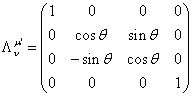
The rotation angle θ is a periodic variable with period 2π. The following is an example of a boost.

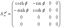
where the boost parameter φ goes from -∞ to ∞.

The boosts correspond to changing coordinates by changing to a frame that is moving at constant velocity with respect to the first frame. The transformed coordinates are given by

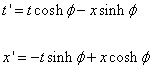
t’ = t cosh φ – x sinh φ

x’ = -t sinh φ + x cosh φ

If the point defined by x’ = 0 is moving, its velocity is given by

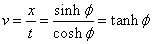
v = x/t = sinh φ/cosh φ = tanh φ

If you replace

φ = tanh^-1 v

you get

t’ = γ (t – vx)

x’ = γ (x – vt)

where

γ = 1/([squareroot of [ 1 – v²)]]

If you don’t use naturalized units where c = 1, then

γ = 1/[squareroot of [1 – (v/c)²)]]

Let’s look at a boost in the x-t plane.

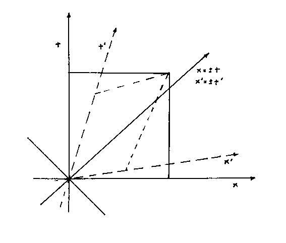
The spacetime axes are rotated into each other, although they do no remain orthogonal. Notice that the path traveled by the light is exactly the same in the new coordinate system as the old one, showing light travels at the same speed for all observers.

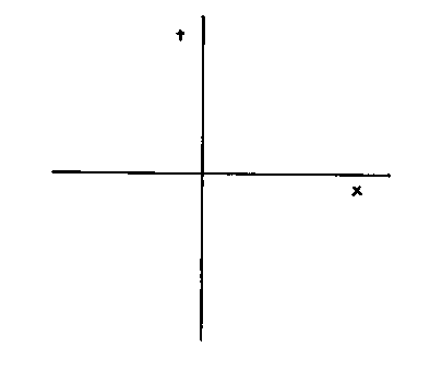
Einstein first presented special relativity in 1905. Then in 1908, Russian mathematician H. Minkowski presented a paper called “Space and Time” in which he introduced the Minkowski diagram. Let’s say you have one dimension of time, and one dimension of space.

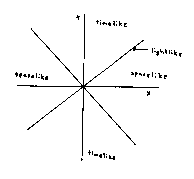
In units where c = 1, the path traced by light passing through the origin would be two lines at right angles to each other, and at 45° angles to the x and t axes. These two lines are called the light-cone, since they would form two cones in an x-y-t system. Points on the lines are called light-like or null. Points above and below the two lines are called time-like. Points to the right and left of the two lines are called space-like. Using the area outside the light-cone as a coordinate frame is called Rindler space.

The spacetime interval is given by

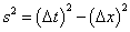
S² = (Δt)² – (Δx)²

And so the interval is zero for

Δx = ± Δt which will only be true if a light-ray can connect the two events since light travels at the speed of one unit of space per one unit of time. Since the interval between points on the light-cone is zero, they are called null.

If the separation between two events A and B is time-like, you can ask if B lies in A’s past or future. The top light cone is A’s future, and the bottom light-cone is A’s past. If the separation between A and B is space-like, you can’t assign an absolute order in time to the events A and B. If two events have space-like separation, some people will say A happens first, some people will say B happens first, and some people will say they are simultaneous. If A and B are time-like separated, then everyone will agree.

The set of points for which the spacetime interval is one would be the unit hyperbola.

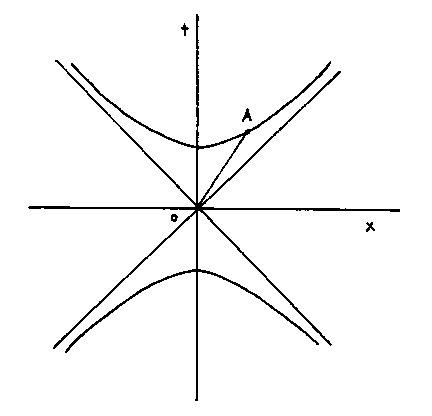
The interval from the origin to A is

1 = t² – x²

You can see that for large values, | t | and | x | are approximately equal and thus the graph is asymptotic to the x = ± t lines.

From the point of view of someone traveling from the origin to A, the 0A line is their t axis. If A has coordinates (x’, t’) in his coordinate system, then x’ = 0. Since the interval 0A is one for every observer

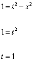
1 = t² – x²

1 = t²

1 = t

so from his subjective point of view, t would appear to take him one time unit to get to any point on the unit hyperbola.

Ironically, some of the assumptions of special relativity are not true in the real Universe. In special relativity, there is no preferred reference frame, but in the real Universe, you could use the cosmic microwave background as a universal reference frame. In special relativity, there is no cosmic time, but in the real Universe, all observers can start their clocks with the Big Bang.

Up until now, we have been assuming that space is flat. This flat spacetime is called Minkowski space, and the equation that defines spacetime intervals in Minkowski space is called the Minkowski metric. We have been discussing special relativity which uses the Minkowski metric which defines flat spacetime. General relativity is a generalization of special relativity to include situations where space is not flat. General relativity includes curved spacetime, and spacetime could be curved like any manifold. I discuss manifolds in more detail in my paper Beyond The Standard Model, at the beginning of the section on string theory. If spacetime is curved, the metric is more complicated than the simple Minkowski metric. First of all, it’s easier to work in spherical coordinates rather than rectangular coordinates.

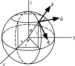
The conversion between spherical and Cartesian coordinates is given by

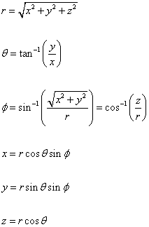
r = [squareroot of (x² + y² + z²)]

θ = tan^-1 (y/x)

φ = sin^-1 ([squareroot of (x² + y²)]/r) = cos^-1 (z/r)

x = r cos θ sin φ

y = r sin θ sin φ

z = r cos θ

You can then define the following line element.

ds = dr[r hat] + rdφ [φ hat] + r sin φ dθ [θ hat]

where the hatted symbols represent the unit vectors. We also want to allow the possibility of any type of curvature, positive, negative, or zero. In the 1920’s, Edwin Hubble measured the redshifts of the galaxies, and determined that the Universe is expanding. Therefore, the metric must also include expansion. The time-dependant scale factor is R(t), and you can make the scale factor dimensionless by defining

a(t) = R(t)/R₀

where R₀ is the current value of the scale factor. In cosmology, the subscript 0 denotes the present era. The scale factor is defined such that at the present era, it’s equal to one.

a(t₀) = 1

Robertson and Walker showed that the only metric consistent with homogeneity and isotropy is

ds² = c² dτ² = g_ij dxⁱ dx^j = c²dt² – a²(t)dl²

where l is lower case “L”, and dl depends only on spatial coordinates. Homogeneity implies that g_tt = 1 giving the first “c²dt²â€ term. This is because all observers can agree on a single time by labeling the time according to a quantity such as density. If everyone agrees that t = 0 when ρ = 100, and t = 10 when ρ = 10, then because of homogeneity, this time will be independent of position. They will all get the same time scale if they each have a clock, and set their clocks according to the Big Bang. Since this registers proper time

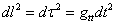
dl² = dτ² = g_ttdt²

Isotropy means there will be no cross terms such as g_x. Therefore, all that is left is to write the spatial element dl.

Let’s look at the case of a sphere. The surface of a sphere is two-dimensional, even though the entire sphere is three-dimensional. A sphere is a 2D space of constant radius of curvature R_c, embedded in 3D Euclidean space, and has a line element of the form

dl² = dx² + dy² + dx²

and in addition, you have the restriction that

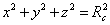
x² + y² + z² = R_c²

Next switch to cylindrical polar coordinates (r, θ, z)

r² = x² + z²

then the line element is

dl² = dr² + r² dθ² + dz²

You also have the restriction that

r² + z² = R_c²

which upon differentiating gives

rdr + zdz = 0

You can then get rid of the dz by differentiating using

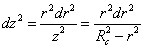
dz² = (r²dr²)/z² = (r²dr²)/(R_c² – r²)

Therefore you have

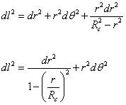
dl² = dr² + r²dθ² + (r²dr²)/(R_c² – r²)

dl² = dr²/(1 – (r/R_c)²) + r²dθ²

You can then make the following transformation.

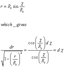
r = R_c sin X/R_c

which gives

dr/[squareroot of (1 – (r/R_c)²)] = (cos (X/R_c)dX)/(cos (X/R_c)) = dX

That is for a sphere with a 2D surface. Now, you simply do the exact same thing for a hypersphere with a 3D surface. In Euclidean 4D space, the line elements is

dl² = dx² + dy² + dz² + dw

with the following restriction

x² + y² + z² = R_c²

Then you have

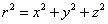
r² = x² + y² + z²

The line element can be decomposed into the usual form in spherical polar coordinates (r, θ, φ) plus the new dimension.

dl² = dr² + r²(dθ² + sin²θdφ²) + dw²

The equation of the hypersphere becomes

r² + w² = R_c²

If you differentiate the equation of the hypersphere, you get

rdr + wdw = 0

and so

dl² = dr² + r²(dθ² + sin²θ dφ²) + ((r²dr²)/(R_c² – r²))

Thus the line element for a 3D space of constant positive curvature 1/R_c² is given by

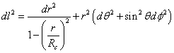
dl² = dr²/(1 – (r/R_c)) + r² (dθ² + sin² θ dφ)

Now we have dl, you can then get the metric.

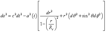
ds² = c²dt² – a²(t) [dr²/(1 – (r/R_c)) + r² (dθ² + sin² θ dφ)]

You can define k = 1/R_c so you have

ds² = c²dt² – a²(t) [dr²/(1 – kr²) + r² (dθ² + sin² θ dφ)]

which can also be written in the opposite sign convention, and in units where c = 1, so

ds² = -dt² + a²(t) [dr²/(1 – kr²) + r² (dθ² + sin² θ dφ)]

This is the Robertson-Walker metric, derived in general by H. P. Robertson in 1935, and A. G. Walker in 1936. The constant k can have values of –1, 0, or 1, which represent the following types of curvature.

k = -1 represents negative curvature, such as a saddle surface or hyperbolic geometry.

k = 0 represents zero curvature, called flat geometry.

k = + 1 represents positive curvature, such as spherical geometry.

There are many different ways of writing down the Robertson-Walker metric. Another useful form is

ds² = c²dt² – a²(t) [dr² + S_k²(r) (dθ² + sin²θ dφ)]

where the function S_k(r) is defined as follows.

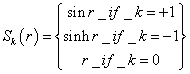
S_k(r) = sin r if k = +1

S_k(r) = sinh r if k = -1

S_k(r) = r if k = 0

You can also define the following function.

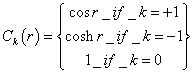
C_k(r) = cos r if k = +1

C_k(r) = cosh r if k = -1

C_k(r) = 1 if k = 0

For k = 0 and k = -1, the radial variable r can take any value from zero to infinity. However, for k = +1, r = π is the equivalent of an opposite pole of the sphere in the 2D case. Larger values of r just go around the sphere to the other side. Therefore, k = +1 is called a closed universe while k = -1 is called an open universe. Of course, k = 0 is also technically open but is called a flat universe. This just means the line element in flat. The metric is not necessarily Minkowskian.

Closed universes have finite volume, but no boundary, like the surface of a sphere. Now, we’ll show how to calculate the volume. The proper distance in the radial direction

dl = [squareroot of -ds²]

with dt = 0 is

dl = R(t)dr

The form of the spherical polar angles in the metric is the same as the Euclidean, which is what you would expect since it’s isotropic. Integrating over them gives 4π steradians, so the proper volume element between shells χ to χ + Δχ is

dV = 4πR³(t)S_k²(r)dr

so then the total volume is

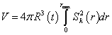
V = 4φR³(t)[integral from 0 to r_max]S_k²(r)dr

For k = 0 or k = -1, r_max = ∞ so the volume is infinite. For k = +1, r_max = π, so you have

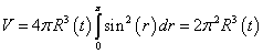
V = 4πR³(t)[integral from 0 to π]sin²(r)dr = 2π²R³(t)

which is finite. It looks like it would be possible in a closed universe to set off in one direction, fly straight without turning around, circumnavigate the universe, and eventually return to the same location from which you left. However, if you take into account the expansion of the universe, this would not be possible.

You should also not confuse the entire Universe with the observable universe, which is a sphere centered on us, with a radius of the horizon distance, which is the length that light could have traveled since the Big Bang. The observable universe is finite. The entire Universe may or may not be finite. The current evidence points to a flat universe, in which such case, it would be infinite. This also relates to common confusion regarding the Big Bang. The observable universe gets larger as time goes on, and thus began as a single point, but if the entire Universe is infinite, it was always infinite, and was not a single point at the Big Bang.

So, the following are all forms of the Robertson-Walker metric.

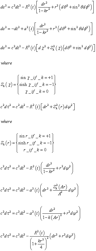
ds² = c²dt² – R²(t)[dr²/(1 – kr²) + r²(dθ² + sin²θdφ²)]

ds² = -dt² + a²(t)[dr²/(1 – kr²) + r²(dθ² + sin²θdφ²)]

ds² = c²dt² – R²(t)[dχ² + S_k²(χ)(dθ² + sin²θdφ²)]

where

S_k(χ) = sin χ if k = -1

S_k(χ) = sinh χ if k = -1

S_k(χ) = χ if k = 0

c²dτ² = c²dt² – R²(t)[dr² + S_k²(r)dψ²]

where

S_k(r) = sin r if k = 1

S_k(r) = sinh r if k = -1

S_k(r) = r if k = 0

c²dτ² = c²dt² – R²(t)(dr²/(1 – kr²) + r²dψ²)

c²dτ² = c²dt² – a²(t)(dr² + ((S_k²(Ar))/A²)dψ²)

c²dτ² = c²dt² – a²(t)((dr²/(1 – k(Ar))²) + r²dψ²)

c²dτ² = c²dt² – ((R²(t))/(1 + (kr²)/4)²)(dr² + r²dψ²)

where A is a constant of proportionality which is equal to R₀, which is equal to the current value of R(t). The last one is called the isotropic form. Also, with any of these, you can define the conformal time in order to take R² out of the metric.

η = [integral from 0 to t]cdt’/R(t’)

In my paper on tensors, I define the Christoffel symbols, Ricci tensor, and curvature scalar. I now define these quantities for the Robertson-Walker metric. Overdots represent derivatives with respect to time. The Christoffel symbols are given by

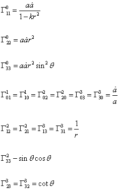
Γ₁₁⁰ = a[a dot]/(1 – kr²)

Γ₂₂⁰ = a[a dot]r²

Γ₃₃⁰ = a[a dot]r²sin²θ

Γ₀₁¹ = Γ₁₀¹ = Γ₀₂² = Γ₂₀² = Γ₀₃³ = Γ₃₀³ = [a dot]/a

Γ₂₂¹ = -r(1 – kr²)

Γ₃₃¹ = -r(1 – kr²)sin²θ

Γ₁₂² = Γ₂₁² = Γ₁₃² = Γ₃₁³ = 1/r

Γ₃₂² = -sin θcosθ

Γ₂₃³ = Γ₃₂³ = cot θ

The non-zero components of the Ricci tensor are

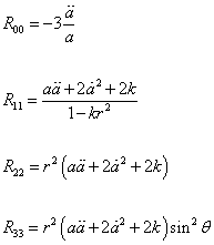
R₀₀ = -3[a double dot]/a

R₁₁ = (a[a double dot] + 2[a dot]² + 2k)/(1 – kr²)

R₂₂ = r²(a[a double dot] + 2[a dot]² + 2k)

R₃₃ = r²(a[a double dot] + 2[a dot]² + 2k)sin²θ

And the curvature scalar is

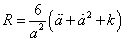
R = (6/a²)(a[a double dot] + [a dot]² + k)

The energy-momentum tensor of a perfect fluid is

T_uv = (p + [rho])U_uU_v + pg_uv

Where [rho] is density, p is pressure as measured in the rest frame, and U^u is the four-velocity of the fluid. Perfect fluids are isotropic in their rest frame. If a fluid is isotropic in some frame, and leads to a metric that is isotropic in some frame, the two frames will coincide, and the fluid will be at rest in comoving coordinates. The four velocity is then

U^u = Diag[1, 0, 0, 0]

And the energy momentum tensor is

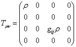
which then becomes

T_v^u = Diag[-[rho], p, p, p]

The trace is given by

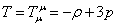
T = T_u^u = -[rho] + 3p

The following is the conservation of energy equation

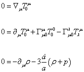
0 = [nabla]_uT₀^u

0 = [partial derivative]_uT₀^u + &Gamma_u0^uT₀⁰ – Γ_u0^λ

0 = -[partial derivative]₀[rho] – 3([a dot]/a)([rho] + p)

The following is the equation of state

w = [rho]/p

The conservation of energy equation becomes

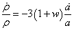
[rho dot]/[rho] = -3(1 + w)([a dot]/a)

which can be integrated to get

[rho] is proportional to a^{-3(1 + w)}

There are three main things in the Universe, which are matter, radiation, and vacuum, which have the following equations of state.

Matter – w = 0

Radiation – w = 1/3

Vacuum – w = -1

Matter is nonrelativistic massive particles for which the pressure is negligible, such as stars and galaxies. Radiation includes both massless particles and massive particles moving relativistically.

The energy density of matter falls off as

p proportional to a^-3

This is the decrease in the number density of particles as the universe expands. The energy-momentum tensor of electromagnetic radiation is

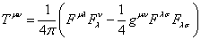
T^μν = -(1/4π)(F^μλF_λ^ν – (1/4)g^μνF^λσF_λσ

The trace of this is given by

T^μ_μ = 1/(4π)[F^μλF_μλ – (1/4)(4)F^λσF_λσ] = 0

This has to be equal to the energy-momentum tensor of a perfect fluid.

T_uv = (p + [rho])U_uU_v + pg_uv

So therefore, the equation of state is

p = (1/3)[rho]

The energy density in radiation falls off as

p proportional to a^-4

The energy density of radiation falls off faster than that of matter because not only does the density of photons decrease but also the individual photons loose energy as 1/a as they redshift.

The Einstein equation with a cosmological constant is

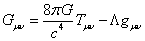
G_uv = (8πG/c⁴)T_uv – Λg_uv

and if you get T_μν on one side, you have

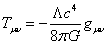
T_μν = -(Λc⁴/8πG)g_μν

This has the form of a perfect fluid with

ρ = -p = Λc⁴/8πG

so therefore, you have w = -1, and the energy density is independent of a, which is what you would expect since the density of the vacuum is always the same. As the universe expands, energy in radiation decreases fastest, energy is matter decreases second fastest, and energy in vacuum does not decrease. Therefore, if you have a nonzero positive cosmological constant, as the universe expands, the universe will begin as radiation-dominated, pass through a matter-dominated stage, and end up as vacuum-dominated. The non-zero vacuum energy tends to win out over the long term, as long as the universe keeps expanding. Today, the contribution to the energy density of the Universe is about 0.3 matter, 0.7 vacuum, and 10^-6 radiation. It’s a puzzle why the contribution from matter and the contribution from the vacuum are within an order of magnitude. Throughout most of the history of the Universe, both past and future, they will not be so close. The Universe was radiation-dominated until about 10,000 years after the Big Bang, and then was matter-dominated until recently when it started going through a transition from matter-dominated to vacuum-dominated.

Now take the energy-momentum tensor and decompose it. The μν = 0 equation is

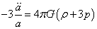
-3([a double dot]/a) = 4πG(ρ + 3p)

Due to isotropy, there is only one distinct μν = ij equation, which is

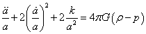
([a double dot]/a) + 2([a dot]/a)² + 2(k/a²) = 4πG(ρ + p)

Take the first of the above two equations, and eliminate the second derivatives in the second one, and you end up with

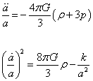
[a double dot]/a = -4πG/3 (ρ + 3p)

([a dot]/a)² = (8πG/3)ρ – (k/a²)

There are called the Friedman equations. Robertson-Walker universes that obey the Friedman equations are called Friedman-Robertson-Walker universes. These models were first studied in 1922 and 1924 by Alexander Friedman, and independently by Georges Lamaitre in 1927. Alexander Aleksandrovich Friedman (1885 – 1925) lived in St. Petersberg, later Leningrad. Since he spelled his name in Cyrillic, there are different ways to transliterate it into English, so you see it spelled Fridman, Friedmann, Friedman, or Freedman.

Remember Hubble’s Law is v = Hd, where Hubble’s constant, more accurately called Hubble’s parameter since it does vary, is given by

H = [a dot]/a

In other words, you could think of it as the rate that two galaxies are moving apart divided by the distance between them. The current value of the Hubble’s parameter is called Hubble’s constant, H₀. Based on WMAP data, the current best guess for the value of the Hubble constant is 0.72 ± 0.5 or 72 km/sec/Mpc, where Mpc is megaparsec, and is equal to 3 x 10²⁴ cm.

The following is the deceleration parameter which measures the rate of change in the rate of expansion.

q = -(a[a double dot]/[a dot]²)

One of the most commonly used quantities in cosmology is the density parameter.

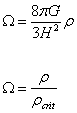
Ω = (8πG/3H²)ρ

Ω = ρ/ρ_crit

where the critical density is defined as

ρ_crit = 3H²/8πG

You can then define the following density parameters in terms of their fraction of the critical density.

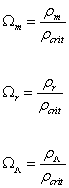
Ω_m = ρ_m/ρ_crit

Ω_r = ρ_r/ρ_crit

Ω_Λ = ρ_Λ/ρ_crit

where

Ω = Ω_m + Ω_r + Ω_Λ

The matter density can be further decomposed into baryonic and dark matter

Ω_m = Ω_b + Ω_d

The current values, based partly on WMAP data are

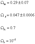
Ω_m = 0.29 ± 0.07

Ω_b = 0.047 ± 0.0006

Ω_Λ = 0.7

Ω_r = 10^-6

so you have about

Ω = Ω_m + Ω_Λ = 0.3 + 0.7 = 1

The density parameters are

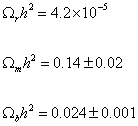
Ω_mh² = 0.14 ± 0.02

Ω_bh² = 0.02 ± 0.0001

Ω_rh² = 4.2 x 10^-5

The Friedman equation says

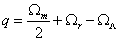
q = Ω_m/2 + Ω_r – Ω_Λ

where q is the deceleration parameter, so therefore

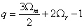
q = 3Ω_m/2 + 2Ω_r – 1

for a flat universe, which could be tested experimentally.

You can use the density parameter to rewrite the Friedman equation.

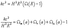
kc² = H² R² (Ω(R) – 1)

kc²/(H²R²) = Ω_m(a) + Ω_r(a) + Ω_Λ(a) – 1

In general relativity, the true source of gravity is not just mass but

ρ + 3p/c = ρ_m + ρ_Λ + 3(-ρ_Λc²)/c² = ρ_m – 2ρ_Λ

The negative pressure of the cosmological constant counter balances the gravitational attraction. The present value of the scale factor can be read from the Friedman equation.

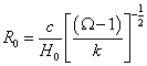
R₀ = (c/H₀)[(Ω – 1)/k]^{– ½}

The Hubble constant sets the curvature length, which becomes infinitely large as Ω approaches unity from either direction. Only in the limit of zero density, does the curvature length equal the Hubble length, c/H₀.

Let’s look at the following equation.

Ω – 1 = k/H²a²

If Ω is more than one, then k is positive, and the universe is closed. If Ω is less than one, then k is negative, and the universe is open. If Ω = 1, then k = 0, and the universe is flat. Then you have

Critical Density	Density Parameter	k	Curvature
ρ < ρcrit	Ω < 1	k = -1	open
ρ = ρcrit	Ω = 1	k = 0	flat
ρ > ρcrit	Ω > 1	k = +1	closed

It is possible to solve the Friedman equations exactly in simple cases, but it’s more revealing to study its qualitative behavior. Let’s say you have no cosmological constant, and you study universes with positive energy and non-negative pressure.

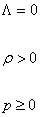
Λ = 0

[rho] > 0

p ≥ 0

Then from

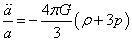
[a double dot]/a = (4πG/3)([rho] + 3p)

The deceleration parameter is always positive. If in this example, the universe can only decelerate, then it would have to be accelerating faster in the past, and if you extrapolate backwards, the universe began in a singularity called the Big Bang. We know that in reality, we have a nonzero positive cosmological constant, and the expansion is accelerating, but it still had to have begun in a Big Bang.

If you still assume no cosmological constant, you can also extrapolate into the future, although the fate of the universe depends on the value of k. In this case, the fate of the universe is actually analogous to firing a rocket on Earth. If the velocity of the rocket is too low, it will be less than the escape velocity. Its trajectory will be a parabola, and it will crash back to the ground. If its velocity is equal to the escape velocity, it will just barely escape, and might go into orbit. If its velocity is higher, it will leave Earth completely, and head off into interplanetary space. You could think of each of these as analogous to different values of k. If k = +1, the universe will not be expanding fast enough to overcome its own gravity. The expansion will slow down, stop, and reverse, and the universe will recollapse and end in a Big Crunch. If k = 0, the universe will be just fast enough for it to escape this fate. If k = -1, the velocity will be higher than that, and it will also expand indefinitely. Therefore, a universe with positive curvature will exist for a finite length of time, while a universe with flat or negative curvature will exist for an infinite length of time. Therefore, universes with k = +1 are both spatially and temporally closed, while universes with k = 0 or k = -1, are both spatially and temporally open.

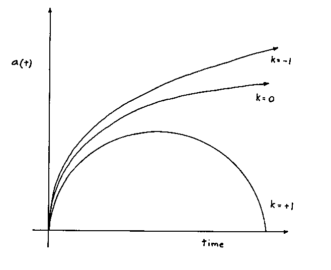
However, remember that this assumes that Λ = 0. With a cosmological constant, you lose the connection between open versus closed, and expand forever versus recollapse. In the real Universe, we have a positive cosmological constant, and so the Universe is spatially flat but the expansion is accelerating.

Now, let’s look at model universes dominated by matter, radiation, and vacuum respectively, and for each one, consider models with k = -1, k = 0, and k = +1.

Matter-dominated, k = -1, open universe

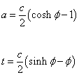
a = (c/2)(cosh φ – 1)

t = (c/2)(sinh φ – φ)

Matter-dominated, k = 0, flat universe

a = (ac/4)^1/3 t^2/3

Matter-dominated, k = +1, closed universe

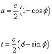
a = (c/2)(1 – cos φ)

t = (c/2)(φ – sin φ)

where φ is the development angle, and is a function of t, and c is a constant defined by

c = (8πG/3) ρ a³

Radiation-dominated, k = -1, open universe

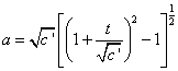
a = [squareroot of c’] [(1 + 1/[squareroot of c’])² – 1]^½

Radiation-dominated, k = 0, flat universe

a = (4c’)^1/4 t^½

Radiation-dominated, k = +1, closed universe

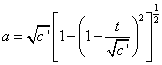
a = [squareroot of c’][1 – (1 – t/[squareroot of c’])²]^½

where c’ is a different constant defined by

c’ = (8φG/3) ρ a⁴

For universes dominated by a cosmological constant, you no longer have the connection between open versus closed and expand forever versus recollapse. If Λ is not zero, it could be either positive or negative. If Λ < 0, Ω is negative, and from that, you get

Ω – 1 = k/H²a²

As you see, this can only happen if k = -1. So for Λ , 0, you can only have k = -1.

Vacuum-dominated, Λ < 0, k = -1, open universe

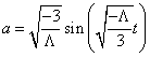
a = [squareroot of (-3/Λ)] sin([squareroot of (-Λ/3)]t)

Vacuum-dominated, Λ > 0, k = -1, open universe

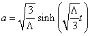
a = [squareroot of (3/Λ)] sinh([squareroot of (Λ/3)]t)

Vacuum-dominated, Λ > 0, k = 0, flat universe

a proportional to e^{± [squareroot of (Λ/3)]t}

Vacuum-dominated, Λ >0, k = +1, closed universe

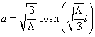
a = [squareroot of (3/Λ)] cosh([squareroot of (Λ/3)]t)

However, it turns out that the last three equations all represent the same spacetime, just in different coordinates. This space, which is the maximally symmetric space with positive cosmological constant, is called de Sitter space. The Λ < 0 solution, which is the maximally symmetric space with negative cosmological constant, and is called anti-de Sitter space.

The deceleration parameter is related to Ω by

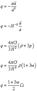
q = -a[a double dot]/[a dot]²

q = -H^-2[a double dot]/a

q = 4πG/3H² (ρ + 3p)

q = 4πG/3H² ρ(1 + 3w)

q = ((1 + 3w)/2)Ω

Since Ω_r is currently negligible, that leaves only two parameters on which Ω depends, Ω_m and Ω_Λ, which can then be graphed on a 2D graphing system. Here I’m drawing it with Ω_m on the horizontal axis, and Ω_Λ on the vertical axis, although sometimes you see it reversed.

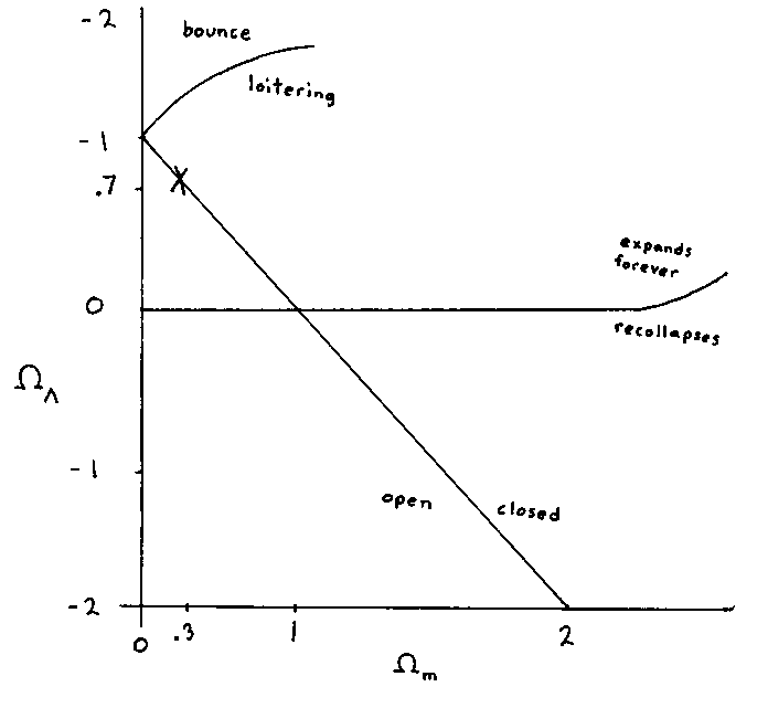
The horizontal line turns up slightly on the right hand side. Above that line, the universe expands forever. Below that line, it recollapses. The diagonal line Ω_m + Ω_Λ = 1, going from upper left to lower right, represents a flat universe. To the right of that line, you have a closed universe with positive spatial curvature. To the left of that line, you have an open universe with negative spatial curvature. In the upper left, you have a region of bounce models, where there was no Big Bang, and instead the universe collapsed from infinity, and before reaching a Big Crunch, instead went through a bounce, and expanded again. Universes on the line in the upper left represent loitering models, where they spend a long time close to a constant scale factor. Both bounce models and loitering models have been ruled out. For a while, we thought that our universe had Ω_m = 1 and Ω_Λ = 0, which is the intersection of the open/closed and expand forever/recollapse lines. However, we now know that the real Universe has Ω_m = 0.3 and Ω_Λ = 0.7, which corresponds to the X on the diagram.

Working out the conditions for these different possible behaviors is simply a matter of integrating the Friedman equation. Ignoring radiation, the time dependant Hubble parameter is

H²/H₀² = Ω_Λ(1 – a^-2) + Ω_m(a^-3 – a^-2) + a^-2

And you look for conditions in which the left-hand side vanishes, defining a turning point in the expansion. Setting the left-hand side to zero gives a cubic equation, and it’s possible to give the conditions under which it has a solution.

Λ < 0 always implies recollapse, which is what you would expect. If Λ > 0 and Ω_m < 1, the model always expands to infinity. If Ω_m > 1, recollapse is avoided only if

Ω_Λ > Ω_m[cos((1/3)cos^-1(Ω_m^-1 – 1) + (4/3)π)]³

If Λ is large enough, the stationary point in the expansion is at a < 1, and you have a bounce cosmology. The critical value is

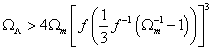
Ω_Λ > 4Ω_m[f((1/3) f^-1(Ω_m^-1 – 1))]³ where

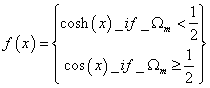
f(x) = cosh(x) if Ω_m < ½

f(x) = cos(x) if Ω_m ≥ ½

If the universe lies exactly on the critical line, the bounce occurred infinitely long ago, and you have a loitering model. These models were briefly popular in the early 1970’s, when it looked like there was a sharp peak in the quasar redshift distribution, but this turned out to be a mixture of evolution and observational selection.

The same cubic equation that defines the critical conditions for the bounce also gives an inequality for the maximum redshift possible in a bouncing universe, which is that of the bounce

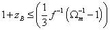
1 + z_B ≤ ((1/3)f^-1(Ω_m^-1 – 1))

so bounce models were ruled out once we had seen objects with redshift z > 2.

If k = 0, it’s called an Einstein-de Sitter model. Since Ω = Ω_m + Ω_Λ = 0.3 + 0.7 = 1 in the real Universe, these models are most relevant to the real universe. The properties of a flat model can usually be obtained by taking the limit Ω -> 1 for either open or closed universes. However, it’s easier to start from the k = 0 Friedman equation.

[R dot]² = (8πGρR²)/3c²

Since both sides are quadratic in R, this makes it clear that the value of R₀ is arbitrary unlike models where Ω is not one. The comoving geometry is Euclidean, and there is no natural curvature scale.

You can therefore work in terms of a normalized scale factor a(t), so that the Friedman equation for a universe with matter and radiation but no cosmological constant is

[a dot]² = H₀²(Ω_ma^-1 + Ω_ra^-2)

which can be integrated to give the time as a function of scale factor

H₀t = (2/3Ω_m²) [[squareroot of (Ω_r + Ω_ma)](Ω_ma – 2Ω_r) + 2Ω_r^3/2]

This goes to (2/3)a^3/2 for a matter-dominated model, and ½ a² for a radiation-dominated model. You can also give the model’s dependence on time.

Matter-dominated universe

t = [squareroot of (1/(6πGρ))]

Radiation-dominated universe

t = [squareroot of (3/(32πGρ))]

You can also look at a k = 0 model with Ω_m + Ω_Λ = 1 with radiation negligible, which is the current Universe. This model allows you to retain k = 0, while varying the age of the universe from H₀t₀ = 2/3 which characterizes the Einstein-de Sitter model.

Ignoring radiation for simplicity, the Friedman equation is

[a dot]² = H₀² [Ω_m a^-1 + (1 – Ω_m) a²)]

and the t(a) relation is

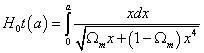
H₀t(a) = [integral from 0 to a]xdx/([Ω_mX + (1 – Ω_m)x⁴

You then use the substitution

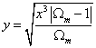
y = [squareroot of ((x³ |Ω_m – 1 |)/Ω_m]

which turns the integral into

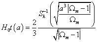
H₀t(a) = (2/3) ((S_k^-1([squareroot of (a³ | Ω_m – 1|)])/Ω_m)/[squareroot of (Ω_m – 1]))

To make it independent of the current era, you can rewrite the equation as

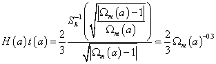
H(a)t(a) = (2/3) ((S_k^-1([squareroot of (| Ω_m(a) – 1|)])/Ω_m)/[squareroot of (Ω_m(a) – 1])) ~ (2/3)Ω_m(a)^-0.3

Up until now, we have been measuring distance with the scale factor a(t). However, of course, in practice, there is no way to measure a(t) directly. In order to relate the theories to the real Universe, you have to express them in terms of quantities that are actually measurable. What you actually observe is the redshift. When you measure light from stars, galaxies, etc., you can measure the tell-tale lines in their atomic spectra. As time goes on, the spectral lines are shifted towards the red end of the spectrum, due to the expansion of the Universe. Imagine a cube containing electromagnetic radiation. As the universe expands, the cube expands, and the electromagnetic radiation gets stretched out.

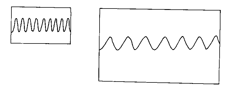
Do you see how the wavelength of the light gets longer, in other words, redshifted? The longer the light has been traveling through space, the longer the length of time since it was emitted, the more the universe has expanded since it was emitted, and so the more the light is redshifted. Therefore, the farther away the source, the more the light is redshifted by the time it reaches us. By measuring the redshift of the light, you can determine how far away the source is. The redshift z is defined as the observed wavelength minus the emitted wavelength, divided by the emitted wavelength, in other words, the fraction the change in the wavelength is of the emitted wavelength. If λ₀ is observed wavelength, and λ_e is emitted wavelength, then

z = (λ₀ – λ_e)/λ_e

z = (λ₀/λ_e) – 1

λ₀/λ_e = a(t₀)/a(t_e)

z = a(t₀)/a(t_e) – 1

a(t₀)/a(t_e) = z + 1

a(t₀) = 1

1/a(t_e) = z + 1

a(t_e) = 1/(z + 1)

Therefore, a(t) is equal to 1/(z + 1).

You can also express the redshift z in terms of frequency instead of wavelength.

ν_e/ν₀ = z + 1

where ν_e is emitted frequency, and ν₀ is observed frequency. Here is the redshift at matter/radiation equality, when matter and radiation made equal contributions to the energy density of the Universe.

z_eg = 3454

Here is the redshift at decoupling, when matter became cool enough for positive ions and electrons to bind into neutral atoms, and so matter decoupled from electromagnetic radiation.

z_dec = 1088

Later, due to the first stars, interstellar hydrogen became reionized, so today, most interstellar hydrogen is ionized. Here is the redshift at reionization.

z_r = 17 ± 5

You must always keep in mind that redshift can also be caused by the Doppler effect, which is a different phenomenon, so you have

1 + z_obs = (1 + z_cos)(1 + z_dop)

However, usually the cosmological contribution to the redshift can be identified. Here you can relate the density parameter to the age of the universe.

t(z) = H(z)^-1{[1- Ω(z)]^-1 + (kΩ(z)/2[k(Ω(z) – 1)]^3/2) C_k^-1[(2 – Ω(z))/Ω(z)]}

where

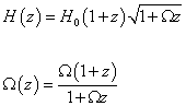
H(z) = H₀(1 + z)[squareroot of (1 + Ωz)]

Ω(z) = Ω(1 + z)/(1 + Ωz)

Using

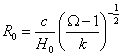
R₀ = c/H₀ ((Ω – 1)/k)^-½

the general relation between commoving distance and redshift is

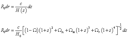
R₀dr = (c/H(z))dz

R₀dr = (c/H₀)[(1 – Ω)(1 + z)² + Ω_Λ + Ω_m(1 + z)³ + Ω_r(1 + z⁴)]^-½dz

For a matter-dominated Friedman model, this means that the distance to an object from which we receive photons today is

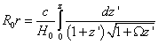
R₀r = (c/H₀)[integral from 0 to z]dz’/((1 + z’)[squareroot of (1 + Ωz’)])

You can solve the integral using the substitution

u² = k(Ω – 1)/Ω(1 + z)

This gives Mattig’s formula, derived by Wolfgang Mattig in 1958.

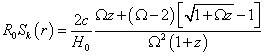
R₀S_k(r) = (2c/H₀)((Ωz + (Ω – 2)[[squareroot of (1 + Ωz)] – 1])/(Ω²(1 + z)))

Another version of Mattig’s formula more convenient for a low-density universe is

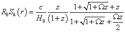
R₀S_k(r) = (c/H₀)(z/(1 + z))(1 + [squareroot of (1 + Ωz)] + z)/(1 + [squareroot of (1 + Ωz)] + (Ωz/2))

Also, it can be written in terms of the function C_k(r) instead of S_k(r).

C_k = ((2 – Ω)(2 – Ω + Ωz) + 4(Ω -1) [squareroot of (1 + Ωz)])/(Ω²(1 + z))

You can extend Mattig’s formula to include contributions from both matter, Ω_m, and radiation, Ω_r.

R₀S_k(r) = (2c/H₀)(Ω_mz + (Ω_m + 2Ω_r – 2)[[squareroot of (1 + Ω_mz + Ω_r(z² + 2z))] – 1])/([ Ω_m² + 4Ω_r(Ω_r + Ω_m – 1)](1 + z))

Unfortunately, there is no equivalent expression that includes vacuum energy, Ω_Λ. The second order distance redshift relation depends on the deceleration parameter.

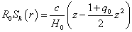
R₀S_k(r) = (2c/H₀)(z – ((1 + q₀)/2)z²)

Since z + 1 is the ratio of the scale factor now and at emission, the redshift will change with time. To calculate the change, differentiate the definition of redshift, and use the Friedman equation. For a matter-dominated model, the result is

[z dot] = H₀(1 + z)(1 – [squareroot of (1 + Ωz)])

The redshift is something we can measure. We know the rest frames of the various spectral lines of the electromagnetic radiation from distant galaxies, so we can tell how much their wavelengths have changed from when they were emitted, t₁, to when they were observed, t₀. Therefore, you know the ratios of the scale factors at these two times. However, we don’t know the times themselves. Since a photon travels at the speed of light, its travel time should be the distance to its source. However, what is the distance to a distant galaxy in an expanding universe? The comoving distance is not measurable, and galaxies need not be comoving in general. In flat space, for a source at distance d, the flux over the luminosity is just one over the area of a sphere centered on the source.

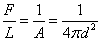
F/L = 1/A = 1/(4πd²)

Using that, you define the luminosity distance as

d_L² = L/4πF

where L is the absolute luminosity of the source, and F is the flux measured by the observer, which is the energy per unit time per unit area. However, in a Friedman-Robertson-Walker universe, the flux will be diluted.

The photons are on average conserved so the total number of photons emitted by the source will eventually pass through a sphere at comoving distance r from the center. Such a sphere is at physical distance d = a₀r from the emitter, where a₀ is the scale factor when the photons are observed. The flux is diluted by two additional effects. The individual photons redshift by a factor (1 + z), and the photons hit the sphere less frequently since two photons emitted at a time Δt apart will be measured at a time (1 + z)Δt apart. Therefore, you have

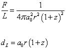
F/L = 1/(4πa₀²r²(1 + z)²)

D_L = a₀r(1 + z)

You can measure the luminosity distance using standard candles, but r is not measurable so you have to remove that from the equation. On a null geodesic chosen to be radial, you have

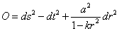
O = ds² – dt² + (a²/(1 – kr²))dr²

which gives

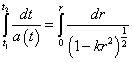
[integral from t₁ to t₀] dt/a(t) = [integral from 0 to r] dr/[squareroot of (1 – kr²)]

You then expand the scale factor in a Taylor series about its present value.

a(t₁) = a₀ + ([a dot])₀(t₁ – t₀) + ½([a double dot])₀(t₁ – t₀)² +…

You can then expand both sides of

[integral from t₁ to t₀] dt/a(t) = [integral from 0 to r] dr/[squareroot of (1 – kr²)]

to find

r = a₀^-1[(t₀ – t₁) + ½H₀(t₀ – t₁)² + …]

Using

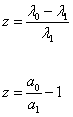
z = (λ₀ – λ₁)/λ₁

z = a₀/a₁ – 1

The Taylor expansion is the same as

1/(1 + z) = 1 + H₀(t₁ – t₀) – ½q₀H₀²(t₁ – t₀)² + …

For small H₀(t₁ – t₀), this can be inverted to give

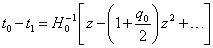
t₀ – t₁ = H₀^-1[z – (1 + q₀/2)z² + …]

substituting into

r = a₀^-1[(₀ – t₁) + ½H₀(₀ – t₁)² + …]

gives you

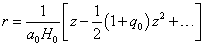
r = (1/a₀H₀) [z – ½(1 + q₀)z² +… ]

Then using

d_L = a₀r(1 + z)

you have

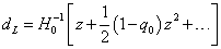
d_L = H^-1[z + ½(1 – q₀)z² + …]

which is another way of writing Hubble’s Law, v = Hd

If you write the Robertson-Walker metric in the following form

c²dτ² = c²dt² – R²(t) [dr² + S_k² (r)dψ²]

then the comoving volume is

dV = 4π [R₀ S_k(r)]² R₀dr

The proper transverse size of an object seen by us is its comoving size dψS_k(r) times the scale factor at the time of emission.

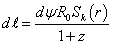
dl = dψR₀S_k(r)/(1 + z)

In order to get the relation between monochromatic flux density and luminosity, you start by assuming isotropic emission, so that photons emitted by the source pass with uniform flux density through any sphere centered on the source. You are free to shift the origin, and consider the Robertson-Walker metric as centered on the source. The photons are then passing through a sphere, where we are located on the surface of the sphere, that has a proper surface area

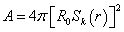
A = 4π[R₀S_k(r)]²

However, the photon energies and arrival times are redshifted, reducing the flux by a factor of (1 + z)². At the same time, the bandwidth dv is reduced by a factor of 1 + z, so the energy flux per unit bandwidth goes down by 1 + z. Also, the observed photons at frequency ν₀ were emitted at frequency ν₀(1 + z), so the flux density is the luminosity at this frequency, divided by the total area, divided by 1 + z.

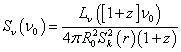
S_ν(ν₀) = L_v([1 + z]ν₀)/4πR₀²S_k²(r)(1 + z)

The luminosity L_ν is measured in units of watts per hertz, W/Hz. Since the emission is not necessarily isotropic, it is common to consider the luminosity emitted into a unit solid angle, in which such case, there would be no factor of 4π, and the units of L_ν would be watts per hertz per steradian, WHz^-1sr^-1.

The specific intensity I_ν is the flux density received from a unit solid angle of the sky

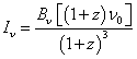
I_ν(ν₀) = B_ν[(1 + z)ν₀]/(1 + z)³

where the surface brightness B_ν is the luminosity emitted into unit solid angle per unit area of source. The flux density received by an observer is the product of the specific intensity and the solid angle subtended by the source.

S_ν = I_ν dΩ

You can integrate over ν₀ to obtain the corresponding total or bolometric formulae.

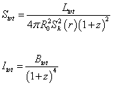
S_tot = L_tot/(4πR₀S_k²(r)(1 + z)²)

I_tot = B_tot/(1 + z)⁴

From this, you can define the angular diameter distance

D_A = R₀S_k(r)/(1 + z)

and the luminosity distance

D_L = R₀S_k(r)(1 + z)

The following is called the effective distance.

R₀S_k(r) = (c/H₀)(2/(Ω²(1 + z))[Ωz + (Ω – 2)([squareroot of (1 + Ωz)] – 1)

Up until this point, we have discussed two possible metrics, the Minkowski metric and the Robertson-Walker metric. However, there are hundreds of obscure metrics that make an appearance in cosmology. It’s common in cosmology papers for the authors to introduce a metric for whatever model they are proposing. Also, any one metric can be written in different ways in different coordinates depending on which is most convenient for the task at hand. However, there are only a few that are used frequently. Here are some commonly used metrics.

Minkowski metric

s² = -(Δt)² + (Δx)² + (Δy)² + (Δz)²

Robertson-Walker metric

ds² = -dt² + a²(t) [dr²/(1 – kr²) + r² (dθ² + sin² θ dφ)]

Schwarzchild metric

ds² = -(1 – 2GM/r)dt² + (1 – 2GM/r)^-1dr² + r²dΩ²

This is the metric of nonrotating uncharged black holes. It was invented by Karl Schwarzschild (1873 – 1916). Notice it reduces to the black holes to the Minkowski metric, when the mass of the black hole is very small, M → 0, or you are very far away from it, r → ∞.

De Sitter metric

Global Coordinates

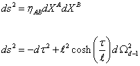
ds² = η_AB dX^A dX^B

ds² = -dτ² – l²cosh(τ/l)dΩ_d-l²

Conformal Coordinates

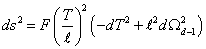
ds² = F(τ/l)²(-dT² + l²dΩ_{d – 1}²)

Planar Coordinates

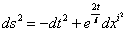
ds² = -dt² + e^2t/ldxⁱ²

Static Coordinates

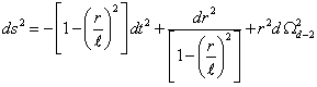
ds² = -[1 – (r/l)²]dt² + dr²/[1 – (r/l)²] + r²dΩ_{d – 2}²

In a strict definition, a universe must have no matter in it, and contain only a positive cosmological constant to be considered a de Sitter universe. However, people usually use a looser definition of de Sitter to mean any maximally symmetric universe with a positive cosmological constant, which would include the real Universe, or at least what the real Universe will evolve into as it becomes increasingly dominated by a positive cosmological constant. A de Sitter universe is often drawn as a hyperboloid in a spacetime diagram.

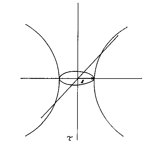
where τ is time, l, which is lower case “L” is the radius, and it contracts from infinity to a finite radius, and expands back to infinity. We are not implying that this diagram represents the behavior of the real Universe, just that’s one way of portraying pure de Sitter space. There are difficulties in making quantum field theory, and thus string theory, consistent with de Sitter space, and since we have evidence for a positive cosmological constant, this is a problem for string theory. Recently, we have come up with an expanded version of M-theory that allowed for de Sitter space, which I discuss at the end of my paper Beyond the Standard Model.

Anti-de Sitter metric

ds² = -Vdt² + V^-1dr² + r²(dθ² + sin²θd&phi²)

where

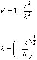
V = 1 + r²/b²

b = (-3/Λ)^½

Anti-de Sitter space is the maximally symmetric space with negative cosmological constant. Although our Universe is obviously not anti-de Sitter, since it has a positive cosmological constant, anti-de Sitter space is important in string theory. In 1997, Juan Maldacena proposed Anti-de Sitter/Conformal Field Theory, or AdS/CFT correspondence, which says that there is a correspondence between Type IIB string theory compactified on AdS₅ x S⁵ and 4-dimensional supersymmetric Yang-Mills theory with N = 4 supersymmetry. I discuss AdS/CFT, correspondence in more detail in my paper Beyond the Standard Model.

Godel Universe

ds² = -dt² + dρ² + sinh²&rhp;(1 – sinh²ρ)dφ² – 2[squareroot of 2]sinh²ρd + dφ _ dz²

where you have closed time-like curves for constant ρ with

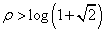
ρ > log (1 + [squareroot of 2]

Originally, the Godel Universe, invented by Austrian mathematician Kurt Gődel (1906 – 1978), was defined as a pressure-free perfect fluid solution in general relativity with negative cosmological constant. It contains closed time-like curves which would allow time travel. Therefore, in order for this model to have anything to do with the real Universe, you would have to get rid of the closed time-like curves. It has been suggested that you could possibly compactify string theory on a Godel Universe, and the holographic principle could possibly get rid of the closed time-like curves. For instance, for supersymmetric backgrounds of the Godel Universe type in string theory and M-theory, a typical example of the metric is

ds² = -dt² + dρ² + ρ²(1 – ρ²)dφ² – 2ρ²dtdφ

as part of the 10d or 11d spacetime. You have closed time-like curves for ρ > 1.

I have to warn you that there is a whole community of crackpots who have latched onto the Godel Universe as their best hope for time travel, just because they think time travel sounds really neat. Unfortunately for them, time travel is intrinsically impossible, and thus any universe that allows time travel is intrinsically impossible. The problem is that time travel, by definition, involves paradoxes, which go under the heading of the grandfather paradox, which is going back in time, and killing your grandfather when he was a young man. This would mean you never existed, which means you couldn’t prevent your existence, so you would exist, which means you could prevent your existence, etc. You just can’t have time travel without paradoxes, and there’s no way around that. Therefore, the Godel Universe is impossible, since it contains closed time-like curves. Unfortunately, the crackpot community have become champions of the Godel Universe, as if the mere invention of a model universe that allows time travel would somehow allow time travel in the real Universe.

Another model universe that does not correspond to the real Universe is the Milne Universe, also called the kinematical model, invented in the 1930’s by British astrophysicist Edward Arthur Milne (1896 – 1950). It used to be an interesting viable alternative to the standard Big Bang model. Its metric is just the Minkowski metric. In traditional cosmology, there is no outside of the universe. The Milne Universe does have an outside. The universe, filled with ready-made galaxies, is created at a single point in flat spacetime. After that, all the galaxies fill the interior of a bubble that expands at the speed of light into previously empty space. It fills the future light-cone of the Big Bang. The galaxies are treated as non-gravitating test particles. We ignore gravity completely. They all shoot out at different speeds along constant velocity straight line paths inside the bubble. The closer they are to the speed of light, the nearer they will be to the surface of the bubble. You have an infinite number of galaxies filling a bubble of finite size. That might sound impossible, but it is possible if you take into account the length contraction of special relativity. In special relativity, an object that moves relative to some reference frame has a reduced length. Its length contracts to zero as its speed approaches the speed of light. The distance between objects is also contracted. The velocity of the galaxies approach the speed of light as you approach the surface of the bubble so you can fit an infinite number of galaxies within a finite bubble. The person traveling at close to the speed of light will not see their own length contracted. Observers in galaxies close to the surface will not notice anything unusual. All the observers in all the galaxies will see basically the same thing, so the Milne Universe is homogeneous and isotropic. This was a very different way of explaining the expansion of the Universe, although it turned out not to be true.

These various metrics of spacetime can be portrayed graphically by the use of Penrose diagrams, where space is the horizontal axis, and time is the vertical axis. Roger Penrose invented his diagrams in order to depict the complete casual structure of any given geometry. Penrose diagrams map everything in the geometry onto a finite diagram, including points at infinite distance, and infinite past and future. Light rays, called null geodesics, are arranged so that they always point 45° from upward vertical.

You begin with a spacetime with physical metric g_uv, and introduce an unphysical metric [g bar]_uv, which is conformally related to g_uv by

[g bar]_μν = Ω²g_μν

where the conformal factor Ω is chosen so as to bring in points at infinity to a finite position so that the whole spacetime is shrunk to a finite region called a Penrose diagram. Here is the Penrose diagram of Schwarzchild spacetime.

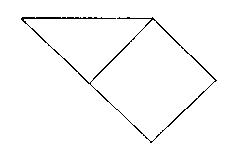
Here is the Penrose diagram for de Sitter space in static coordinates.

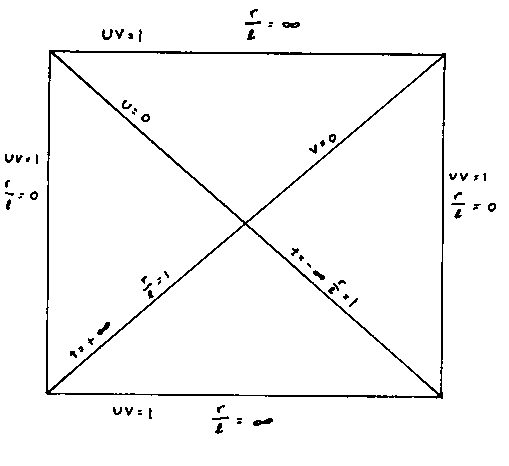
For an observer in any of the four quadrants, the only casual connected region for them in the quadrant that they are in.

From the origin of science in Greece in the 7th Century B.C. up to the 1920’s, it was assumed without question that the Universe had existed forever without beginning. This is despite the fact that Olber’s paradox could be solved by saying the Universe was not infinitely old, but instead the only solution ever suggested was that the Universe was not infinitely large. In 1912, Vesto Slipher measured the redshift of nebulae, which were actually galaxies, and most were redshifted. In 1923 – 1929, Edwin Hubble measured the redshift of the galaxies in detail, which was the first evidence that the Universe had a beginning. There then raged a debate between the Big Bang model and the Steady State model, until the Cosmic Microwave Background was detected in 1964, which was very convincing evidence for the Big Bang model, although a few holdouts continued to cling to the Steady State model. There were some problems with the traditional Big Bang model, such the horizon, flatness, and monopole problems, which were solved by the theory of inflation proposed by Alan Guth and Andrei Linde in 1981. It was later realized that inflation allowed the possibility of eternal inflation, which means the Universe could have existed for an infinite length of time after all, even assuming the Big Bang, so it is still an open question as to whether time extends infinitely backwards or not. Now, the idea that the Universe existed for an infinite length of time poses no problems if you assume that all the stars were printed on the interior surface of the celestial sphere which had existed for an infinite length of time. The celestial sphere was thought to be made out an indestructible crystalline material that could last forever. This cosmological model held the unanimous consensus among physicists and astronomers from the 7th Century B.C. to the 1570’s. Then in 1576, English astronomer Thomas Diggs suggested that there was no celestial sphere, and instead that stars were scattered randomly throughout a huge three dimensional volume of space, perhaps infinitely large. This became the majority view. However, this then posed a problem when combined with Newtonian mechanics, and the assumption that the Universe had existed for an infinite length of time. In Newtonian classical mechanics, all matter attracts all other matter through gravity. Therefore, all the stars would gravitationally attract each other. Given enough time, all the matter in the Universe would collapse together under its own gravity. If the Universe was infinitely old, there would obviously be enough time for this to happen. Instead of interpreting this as evidence against an infinitely old universe, Newton solved the problem by postulating that there existed some sort of repulsive force that counteracted the attraction of gravity. This was the very first suggestion of a cosmological constant. This is the exact same rationale that Einstein used for suggesting a cosmological constant. When Einstein invented general relativity in 1917, it after Slipher first measured the redshift of galaxies but before Hubble’s detailed survey of the redshift of galaxies in the 1920’s, so there was no compelling evidence that the Universe had not existed for an infinite length of time. In physics, you try to think up a theory that explains what you observe. This is exactly what Einstein did when he came up with a model that fit what they observed, which at the time was a stable universe. Therefore, Einstein proposed a cosmological constant that would provide a negative pressure to the universe to counteract the attractive force of gravity.

The problem is that Einstein’s trick of using the cosmological constant to try to make the universe static does not work. Einstein’s model is unstable even with a cosmological constant. Let’s say you have a universe with both matter and vacuum energy. The gravitational attraction of the matter will work to contract the universe. The repulsive effect of the vacuum energy will work to expand the universe. Now, if these two effects cancel each other out exactly, you have a static universe. Now, let’s say you make the universe ever so slightly smaller. Then the matter density will be slightly higher, and thus the gravitational attraction will be slightly higher, but the vacuum density, as always, will be exactly the same, so the repulsive effect will be the same. That means the gravitational attraction and the repulsive effect from the vacuum will no longer cancel each other out, and you’ll have a net gravitational attraction. A net gravitational attraction will cause the universe to contract further, making the matter density even higher, and thus the gravitational attraction even higher. The vacuum energy will be exactly the same so the discrepancy between the magnitude of the gravitational attraction and the repulsive effect of the vacuum energy even greater. This will cause the universe to contract even more. As you see, this sets up a positive feedback loop. Just making the universe just the tiniest possible amount smaller will eventually lead to the entire universe collapsing completely. You also have the same thing in the opposite direction. If you make the universe just slightly larger, the matter density will be slightly lower, and so the gravitational attraction will be slightly lower. The vacuum density will still be exactly the same, so the repulsive effect of the vacuum energy will still be the same. Then the gravitational attraction will not be enough to compensate for the repulsive effect of the vacuum energy, so you will be left with a net repulsion due to the vacuum energy. This will cause the universe to expand even larger, which will cause the matter density to decrease further, which will cause the gravitational attraction to decrease further. Again, you have a feedback loop, and the universe will expand forever. So you see, Einstein’s model of the universe is unstable. The tiniest possible deviation from total perfect cancellation will be exaggerated over time. The tiniest perturbation leads to either contraction or expansion. Therefore, Einstein’s model universe was not stable, and the cosmological constant did not make it stable. Einstein failed to create a static universe but it took several years for people to realize this. In 1930, Eddington showed that Einstein’s model was unstable.

In 1917, before the galactic redshifts were generally known, Einstein proposed a model universe in which random galactic motions cancel out, leaving it static. The mean density of the universe remained constant over time. The radius of the universe remained constant over time. It was a closed universe with spherical geometry. It was finite with no center and no boundary. Einstein then introduced a cosmological constant which was a small repulsive force between matter. This force acts over intergalactic distances and keeps the model from collapsing under its own self-gravitation. In Einstein’s static model, the radius is inversely proportional to the squareroot of the mean density of matter. The mean density is estimated to be between 10^-29 and 10^-31 g/cm³. This would predict a radius of the universe between 10¹⁰ and 10¹⁰⁰ light-years. Of course, the observable universe only has a radius of 13.7 billion light-years, since the Universe is 13.7 billion years old. In 1930, Eddington showed that Einstein’s model is actually unstable, and should either expand or contract if perturbed. In 1917, Dutch astronomer William de Sitter (1872 – 1934) proposed another apparently static model, although his model turned out not to be static either. His model contained no matter. It was not really static, and was the forerunner of expanding models. It predicted expansion would last forever. It predicted redshift proportional to distance.

In 1930, Eddington in England proposed a nonstatic model. His model was simply a perturbation of Einstein’s static model. It begins an expansion that lasts forever. Also in 1930, Belgian priest George Lamaitre (1894 – 1966) proposed a nonstatic model. Lamaitre’s model begins with a Big Bang, expands for a while, hesitates in a state resembling Einstein’s static universe, and then expands a second time, and then expands forever. Lamaitre was called the “father of the Big Bang”. In 1922, Russian cosmologist Alaxander Friedman (1888 – 1925) derived nonstatic models that predicted galactic redshifts. His models went unnoticed in the scientific community. According to the Friedman equation, if you assume a mean density equal to the critical mean density, the amount of matter is precisely such that mutual gravitational attraction will stop the expansion when the universe is of an infinite size. This is called a flat or marginally open model. If the mean density is greater than the critical density, the expansion will stop at a finite size, the radius of which is determined by the amount of matter, and is called a closed model. Any value of mean density greater than the critical density, produces one of an infinite family of cosmological models. If the mean density is less than the critical density, even when space becomes infinite, the expansion continues, and is called an open model. Any value of mean density less than the critical density, produces one of an infinite family of cosmological models. In these models, the cosmological constant could be positive, negative, or zero, but non-zero values greatly increase the number of models, and some people believed that the mere proliferation of models argued that the cosmological constant was zero. In 1935, A. G. Walker and H. P. Robertson independently proved that what we now call the Robertson-Walker metric is the only metric consistent with a homogeneous isotropic universe.

In 1912, Vesto Slipher started measuring spectra from nebulae that showed that many appeared to be Doppler shifted, meaning that the frequency of the light was affected by the speed of the source. By 1924, 41 nebula had been measured, and 36 of these were found to be receding. In 1923 – 1929, Erwin Hubble did a more detailed study of galactic redshifts, and determined the proportionality between velocity and distance. Hubble was able to resolve Cepheids in M31, the Andromeda Galaxy, with the 100-inch telescope at Mount Wilson. He developed a new distance measure using the brightest star for more distant galaxies. He correlated these measurements with Slipher’s nebula to discover a proportionality between velocity and distance, and came up with Hubble’s Law, v = Hd. Hubble’s constant H was significantly overestimated by Hubble himself. Here is a plot of Hubble’s 1929 data of radial velocity plotted versus distance.

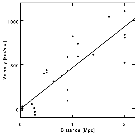
The slope of the tilted line is 464 km/sec/Mpc. Since both kilometers and megaparsecs are units of distance, the units of Hubble’s constant H₀ can be reduced to 1/t where

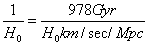
1/H₀ = 978 Gyr/(H₀ in km/sec/Mpc)

According to Hubble’s data, Hubble’s constant would have a value of two billion years which would be the age of the Universe, except they knew from radioactive dating of rocks that the Earth was older than that. This obviously wrong result gave hope to those who preferred the Steady State model. However, it was later realized that Hubble had confused two different kinds of Cepheid variable stars used for calibrating distance, and also some of what Hubble thought were bright stars were actually HII regions. Hubble’s 1929 data was also unreliable since individual galaxies have individual velocities of several hundred km/sec, in addition to the apparent cosmological recession, and Hubble’s data only went out to 1200 km/sec. This led some people to propose quadratic redshift distance laws. However, later improved data confirmed Hubble’s Law. For instance, the following plot uses data collected by Riess, Press, and Krishner in 1996, using supernovae data.

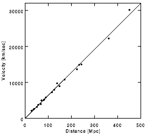
The current estimate of Hubble’s constant based on WMAP data is 0.72 ± 0.05. So as data regarding galactic redshift improved, the evidence for the Big Bang mounted. One thing that’s confusing is that the time and distance used in Hubble’s Law are not the same x and t used in special relativity. Therefore, galaxies far enough away appear to have velocities greater than light. However, they aren’t really traveling faster than light. This is just an artifact of the coordinate system. In 1964, Arno Penzias and Robert Wilson detected the cosmic microwave background. Working with a 7.35 cm microwave horn antenna at Bell Labs, Penzias and Wilson accidentally discovered an isotropic radio background. The cosmic microwave background radiation is key evidence for the hot big bang model. The temperature of this black body radiation is 2.725 K. So you had overwhelming evidence for the Big Bang but there were problems with the traditional Big Bang model. The observable universe is a sphere centered on us, where the radius is the horizon distance, which is the maximum distance light could have traveled since the Big Bang. Thus, the observable universe gets larger as time goes on. Anything within the observable universe is within our past light-cone, and is casually connected to us. Anything outside the observable universe is outside our past light-cone, and is not casually connected to us. If two regions are not casually connected, there is no way they could possibly affect each other. However, when you look to the edge of the observable universe, everything is very similar. The Universe appears homogenous and isotropic, including regions that only recently came within our past light-cone, which means they had to have been very similar before they were casually connected. That sounds impossible. Before they were casually connected, there was no way they could have influenced each other, so what could have made them so similar? This is called the horizon problem.

Another problem is why is the Universe so extremely close to flat? The flatness is indicated by the isotropy of the cosmic microwave background which is isotropic to one part in 10⁵. This is more obvious if you calculate the critical density. The critical density one nanosecond after the Big Bang must have been 447,225,917,218,507,248,016 g/cm³. If you were to add 1 g/cm³ to this, it would cause the Big Crunch to be happening right now. If you were to take 1 g/cm³ away, it would cause Ω to be too low for observations. Therefore, the density one nanosecond after the Big Bang was set to an accuracy of one part in 447 sextillion. At the planck time after the Big Bang, it was set to an accuracy of one part in 10⁶⁰. What would cause the Universe to be so flat? This is called the flatness problem. Another problem is that phase transitions in the early universe cause topological defects such as magnetic monopoles. The Universe should be filled with monopoles yet we’ve never detected one. This is called the monopole problem. It turns out that the horizon problem, flatness problem, and monopole problem can all be solved by a theory called inflation, which was first suggested by Starobinsky, and later developed by Alan Guth and Andrei Linde in 1981. This assumes that the universe went through a period of enormous accelerated expansion right after the Big Bang, much larger than the accelerated expansion it’s undergoing now. Let’s say you had a sphere with a radius of the planck length before inflation, and inflation only lasted for the planck time. After inflation, the sphere would be several orders of magnitude larger than the current observable universe.

Let’s say you have two tiny regions right next to each other before inflation. This is on the planck scale. They would be similar to each other because they are tiny regions right next to each other, and are casually connected. Inflation would blow them up to huge size, but they would still be similar to each other because they were similar before inflation, and would remain so after inflation. You would then end up with regions that are no longer casually connected but still very similar. Also, inflation would blow up any deviation from flatness much larger than our current horizon length, so what’s within our horizon would appear flat. Inflation would flatten the universe. Also, if regions on the planck scale are blown up to be larger than the observable universe, it’s very unlikely that there would be any monopoles within our observable universe. Therefore, inflation solves the horizon, flatness, and monopole problems. So if the expansion of the universe is caused by the repulsive effect of the cosmological constant, and inflationary cosmology assumes an enormously large amount of expansion in the very beginning of the universe, that means that there was a very large effective cosmological constant in the very beginning of the universe. We have a much smaller but still positive cosmological constant today since the expansion of the Universe is still accelerating, which you can tell from the supernovae Ia data.

Standard cosmology contains a particle horizon of comoving radius

r_H = [integral from t to 0] cdt/R(t)

which converges because

R is proportional to [squareroot of t]

in the early radiation-dominated phase. At late times, the integral is determined by the matter-dominated phase

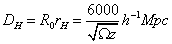
D_H = R₀r_H = 6000/[squareroot of Ωz]h^-1Mpc

The horizon at last scattering, z = 1000, was thus only 100 Mpc in size, subtending an angle of about one degree. How is it then possible that the cosmic microwave background is isotropic to one part in 10⁵ all over the entire sky? This is called the horizon problem.

In a flat Ω = 1 universe

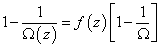
1 – 1/Ω(z) = f(z)[1 – 1/Ω]

where

f(z) = 1/(1 + z)

in the matter-dominated era and

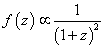
f(z) is proportional to 1/(1 + z)²

in the radiation-dominated era. Therefore

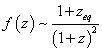
f(z) ~ (1 + z_eq)/(1 + z)²

at early times. To get Ω ~ 1 today requires a fine tuning of Ω in the past which becomes more and more precisely constrained as you increase the redshift, and thus go farther and farther backwards in time. Ignoring annihilation effects, you have

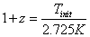
1 + z = T_init/2.725 K

and 1 + z_eq ~ 10⁴, so that the required fine tuning is

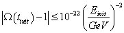
| Ω(t_init) – 1| < 10^-22(E_init/GeV)^-2

If you choose the planck time as the initial time, this requires a deviation of less than one part in 10⁶⁰. What could cause the universe to be as flat as that? This is called the flatness problem.

You can solve the horizon and flatness problems if you assume that there was an interval where the universe appeared to be expanding faster than light. Of course, it’s not really traveling faster than light, and this fact is obvious if you look at special relativistic coordinates. If you had such a phase, the integral for the comoving horizon would have diverged, and then the overall homogeneity could be explained by normal casual processes. You could even say that the observed homogeneity proves that such casual contact must have once existed. This is called inflationary cosmology. A period of inflation requires

[rho]c² + 3p < 0

This causes the active mass density

[rho] + 3p/c²

to vanish. Since this is the right hand side of the Poisson equation generalized to relativistic fluids, it’s not surprising that the vanishing ρ + 3p/c² allows a coasting solution with R proportional to t. Here you have the Friedman equation.

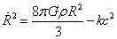
[R dot]² = (8πGρR²/3) – kc²

With inflation, the density term on the right hand side must exceed the curvature term by a factor of 10⁶⁰ at the planck time. An inflationary phase in which ρR² increases as the universe expands can make the curvature term comparatively small.

Inflation requires a state with negative pressure, and the obvious example is p = ρc² which is the vacuum energy. Therefore, inflation happens in a universe dominated by a cosmological constant. The Friedman equation in the vacuum-dominated case has three solutions.

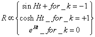
R is proportional to sinh Ht for k = -1

R is proportional to cosh Ht for k = +1

R is proportional to e^Ht for k = 0

where

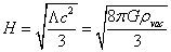
H = [squareroot of (Λc²/3)] = [squareroot of (8πGρ_vac/3)]

All solutions evolve towards the exponential k = 0 solution, which is de Sitter space. In all models, Ω will tend to unity as the Hubble parameter tends to H₀. If the initial conditions are not fine-tuned to Ω = 1, then maintaining the expansion for a factor f gives

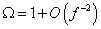
Ω = 1 + O(f^-2)

This can solve the flatness problem if f is large enough. To get Ω = 1 today requires

| Ω – 1 | < 10^-52

at the GUT epoch, and so

ln f > 60

which means 60 e-foldings of expansion are needed to solve the flatness problem which is the same number as needed to solve the horizon problem. Inflation predicts k = 0.

So our current view of the Universe, inflationary cosmology, assumes a large effective cosmological constant in the beginning of the universe, which causes inflation, which solves the horizon problem, flatness problem, and monopole problem, as well as a small positive cosmological constant today, which causes an acceleration of the expansion of the universe, as indicated by the supernovae Type Ia data. An additional benefit of inflation, and thus the cosmological constant, is that you can use it to explain why the Big Bang happened in the first place. The original traditional Big Bang model gave absolutely no explanation as to why the Big Bang itself happened. The Big Bang itself was just taken as an initial condition without explanation. However, if in the beginning of the universe, there was a period of enormous expansion caused by an effective cosmological constant, you might as well include the Big Bang itself in that, so then the Big Bang itself would be caused by a large effective cosmological constant. So then you have a large cosmological constant in the beginning of the universe which causes the Big Bang and inflation, which solves the horizon problem, flatness problem, and monopole problem, and a small cosmological constant today which explains the acceleration of the expansion of the universe as indicated by the supernovae Type Ia data.

Today, we think of the expansion of the Universe as evidence for the cosmological constant. From our point of view today, we would assume that the detection of the redshift of the galaxies proved the existence of the cosmological constant. However, strangely enough, people at the time said the opposite. When the redshift of the galaxies was first detected, people acted like it proved the nonexistence of the cosmological constant. Einstein said that the cosmological constant was “the biggest blunder of my life”. Why is this? You have to look at it from a historical view. Einstein invented the cosmological constant to keep the universe static. Then when it was learned that the Universe wasn’t static, that means you don’t need a thing the purpose of which is to keep the universe static. If the cosmological constant was invented to keep the universe static, and the Universe isn’t static, that means you don’t need a cosmological constant. Of course, that never proved there wasn’t a cosmological constant. There were nonstatic models with a positive, negative, or zero cosmological constant. However, in physics, you choose the simplest explanation. It was believed that a zero cosmological constant was simpler than a nonzero one. They obviously didn’t need a cosmological constant to explain the horizon, flatness, or monopole problems, or the supernovae Ia data, since none of those things had yet been detected or theorized. As far as the Big Bang itself was concerned, they thought asking what caused the Big Bang was like asking what caused the Universe, which they thought sounded like a metaphysical unanswerable question that was outside the domain of physics to even ask about. At any rate, they reasoned if the Big Bang occurred at t = 0, then there was no “before” so there couldn’t have been anything before that caused it.

You can easily add a cosmological constant in an ad hoc way to Einstein’s equation but we would like to have an underlying motivation for it. What actually is the cosmological constant, meaning what actually causes this vacuum energy? One possible explanation comes from particle physics. If you look at the ladder operators for the creation and annihilation operators, the energy is nonzero even when the number of particles is zero. Therefore, the vacuum itself has energy. I explain this in more detail in my paper on the Standard Model. The vacuum is filled with particle-antiparticle pairs continually coming in and out of existence, and they contribute to the vacuum energy.

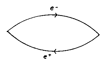
For a particle of mass m, you have one virtual particle in each cubic volume of space, where the length of each side is the Compton wavelength of the particle h/mc, where h is Planck’s constant. The expected energy density is

[rho] = m⁴c³/h³

If you choose m to be the Planck mass, 10¹⁹ GeV, that would give 2 x 10⁹¹ g/cm³. This is 10¹²⁰ times larger than the observed value. This is the largest discrepancy between a theoretically predicted value and an experimentally measured value in all of physics. If you take supersymmetry into account, it is only 10⁵⁵ too large. I explain why in my paper Beyond The Standard Model. Now you can explain this discrepancy if you say that factors we don’t know about cancel each other to give the small net value we detect, which is the premise of renormalization in quantum field theory. In this case, they would have to cancel out to 120 or 55 decimal places. This is possible, but many people feel it is highly unlikely or unnatural. This is called a fine-tuning problem.

You can, of course, just say that the vacuum energy is not the result of particle-antiparticle pairs, and is instead the result of a scalar field rolling down its potential like in the Higgs mechanism. This doesn’t have a fine-tuning problem. Today, it is common to say that the cosmological constant is caused by a scalar field rolling down it’s potential, and is thus not a constant at all but a varying parameter. This rolling scalar field is called quintessence. It is necessary to have some sort of rolling scalar field to explain both the original inflation and the current acceleration of the expansion of the Universe. With a traditional cosmological constant, w = -1. In the quintessence model, the dark energy is associated with a universal quantum field relaxing towards some final state. Here the energy density and pressure of the dark energy are slowly decreasing with time, and the value of w is somewhere between -1/3 and -1, where w must be smaller than -1/3 in order for cosmic acceleration to occur. It has also been suggested that you could have w < -1, called phantom energy, which could cause the universe to end in a Big Rip, in which all matter is eventually ripped apart by vacuum energy.

Up until the 1980’s, most cosmologists took the current cosmological constant to be zero, simply because that would be the simplest model. However, throughout the late 20th Century, there was gradually increasing evidence for a nonzero positive cosmological constant. Mostly, it was indirect. As there were more and more accurate measurements of the amount of matter in the Universe, it became more and more apparent from the isotropy of the CMB, as well as the theory of inflation, that the Universe is very close to flat, and from gravitational lensing, that even including dark matter, the amount of matter in the Universe is not enough to flatten the Universe. Since Ω_m + Ω_Λ = 1, that means if Ω_m < 1, then Ω_Λ 0, in other words, we have a positive cosmological constant. Inflation predicted the universe is flat. Then it was realized that the amount of matter in the Universe was not enough to flatten the universe, which meant we had a cosmological constant, would cause the expansion to accelerate. At first we did not detect any such acceleration, but then we did detect it in supernovae data, and many cosmologists breathed a sigh of relief.

The real proof of a positive cosmological constant was when the acceleration of the expansion of the Universe was detected by studying the redshifts of Type Ia supernovae. It’s notoriously difficult to measure interstellar, much less cosmological, distances. For the nearest stars, you can use triangulation, which is basically what George Washington did as a Public Land Surveyor. For distances farther than that, you have to use standard candles. Apparent brightness equals actual brightness divided by the distance squared. Let’s say you measure the distance to several nearby celestial objects using parallax or some other means. With the distance and their apparent brightness, you can calculate their actual brightness. If the actual brightness turns out to be the same for all the objects of a given type, you can conclude that the actual brightness is always the same for objects of that type, and it is therefore a standard candle. Now let’s say you find celestial objects of that same type too far away for the distance to be measured by any other method. Since you know the actual brightness, and you can measure the apparent brightness, from that you can calculate the distance. Therefore, standard candles are the only way to calculate the distance to distant galaxies. The most famous type of standard candle is Cepheid variables, which are stars for which the brightness is related to the period of the variation in the brightness, so you can calculate the actual brightness. Edwin Hubble used entire galaxies as standard candles but their intrinsic brightness varied widely. As early as 1938, Walter Bade suggested using supernovae as standard candles. For modern cosmology, the main standard candle is Type Ia supernovae. If supernovae have no hydrogen features in their spectra, they are called Type I. If supernovae do have hydrogen features in their spectra, they are called Type II. In the early 1980’s, Type I supernovae were subclassified into Type Ia and Type Ib. If Type I supernovae have a silicon absorption feature at 6150 angstroms in their spectra, they are called Type Ia. If Type I supernovae do not have a silicon absorption feature at 6150 angstroms in their spectra, they are called Type Ib.

A star like the Sun uses up its nuclear fuel in 5 – 10 billion years, and then it shrinks to a white dwarf with its mass, mostly carbon and oxygen, supported against further collapse by electron degeneracy pressure. What if the white dwarf is in a close binary orbit with a large star that is actively burning its nuclear fuel? If conditions are right, there will be a steady stream of material from the active star to the white dwarf. Over millions of years, the white dwarf’s mass builds up until it reaches the critical mass, near the Chandrasekhar limit of about 1.4 solar masses that triggers a runaway thermonuclear explosion called a Type Ia supernova. The slow relentless accretion of material until the characteristic mass is reached erases most of the individual histories and original differences between the stars that collapsed to form the white dwarves. Therefore, the light curves and spectra of all Type Ia supernovae end up being all very similar. Thus, they are excellent standard candles. Since they are bright enough to be seen in the most distant galaxies, they can be used to measure cosmological distances. By measuring both the redshift and the distance of Type Ia supernovae, you can plot redshift versus distance. Two separate teams measured Type Ia supernovae in the late 1990’s. One was the Supernova Cosmology Project led by Saul Perlmutter of Berkeley. The other was the High-Z Supernovae Search led by Brian Schmidt of Australia’s Mount Stromlo Observatory. The results of the two teams confirmed each other.

Type Ia supernovae are very bright and very regular, and can be used as standard candles all the way out to the most distant observable galaxies, and thus can be used to measure the expansion rate of the Universe. However, there were difficulties in using them. First of all, they are rare. A typical galaxy only has a few Type Ia supernovae per millennium. Second of all, they are random, giving no advance warning of where to look. The scarce observing time at the world’s most powerful telescopes is allocated on the basis of proposals written six months in advance. Even the few successful proposals are granted only a few nights a semester. Third of all, they are fleeting. After exploding, they must be observed immediately, and measured multiple times within a few weeks, or they will have already passed the peak brightness that is essential for calibration. You couldn’t preschedule telescope time to identify a supernova’s type or follow it up if you couldn’t guarantee a Type Ia supernova. At the same time, you couldn’t prove a technique for guaranteeing Type Ia supernovae discoveries without prescheduling telescope time to identify them spectroscopically. Eventually, Saul Perlmutter and his team solved this problem. They built a wide-field imager for the Anglo-Australian Observatory’s 4-meter telescope. The imager allowed them to study thousands of distant galaxies in one night, greatly increasing the likelihood of a supernova discovery. By specific timing of the requested telescope schedules, they could guarantee that their wide-field imager would harvest a batch of about a dozen recently exploded supernovae, all discovered on a pre-scheduled observing date during the dark phases of the Moon, which is the best time to do astronomy.

The Supernova Cosmology Project first presented its results in 1997, and it seemed to suggest that the expansion was slowing, but it still had large error bars. In 1998, both the Supernova Cosmology Project led by Saul Perlmutter, and the High-Z Supernova Search, led by Brian Schmidt, presented results that showed that the expansion was accelerating. This proved that we had a non-zero cosmological constant. This should not have been surprising because theoretical cosmologists, such as Michael S. Turner, had long predicted that we had a positive cosmological constant, and should be seeing such an accelerated expansion. By 1990, estimates of the amount of dark matter were getting better but still falling short of enough to flatten the Universe. Observations of large scale structure suggested a cold dark matter or CDM universe with a matter density about one third the critical density, or Ω_m = 1/3. Inflationary cosmology predicted a flat universe, or Ω = 1, which is consistent with the isotropy of the cosmic microwave background. Since Ω_m + Ω_Λ = 1, and Ω_m = 1/3, that means Ω_Λ = 2/3. That means we have a positive cosmological constant which would cause an acceleration of the expansion. Therefore, the theoretical cosmologists had long been saying that we should observe what the two supernovae teams did observe. The theoretical cosmologists breathed a sigh of relief when the acceleration was finally detected. Despite that, Saul Perlmutter, Brian Schmidt, and their teams were so flabbergasted, they just didn’t believe what they were seeing. They just refused to believe their own data. They assumed it was an experimental error. They went over their own data dozens of times, trying to find the source of the error. If two separate teams had not independently reached the same result, they never would have believed it.

This doesn’t make any sense because according to our theories, we should be observing exactly what they observed. It was predicted ahead of time. The supernovae Type Ia data was a confirmation of what our theories predicted we should be observing. Why then were the teams so surprised by this, to the point of disbelieving their own data? If you study physics as I have, you begin to notice that in all fields of physics there is a major communication gap between the theorists and the experimentalists. These are usually very separate communities. This problem seems to be especially pronounced in cosmology. For instance, the cosmic microwave background was predicted in 1949 by Alpher and Herman. Despite that, when it was finally detected in 1964 by Penzias and Wilson, they didn’t know what it was. They assumed it was some sort of problem with their equipment. They even went so far as to try to clean the pigeon shit out of their microwave antennae in order to try to get rid of the annoying background buzz. Similarly, cosmologists like Micheal Turner had predicted in 1990 that we should be observing an acceleration in the expansion due to a positive cosmological constant. This should be easy enough for anyone to understand. If the universe is flat, Ω = 1, and according to observations of large scale structure, Ω_m = 1/3, which means Ω_Λ must be 2/3. Therefore, the expansion should be accelerating. Despite that, when it was finally detected in 1998 by Saul Perlmutter and Brian Schmidt, they just couldn’t believe it. They assumed it was a systematic error. They went over their data over and over again trying to find the mistake. If two teams hadn’t come up with the same result, they never would have believed it. Perhaps this is because decades earlier it had been assumed for simplicity that we had zero cosmological constant, so that’s probably what they were taught in school, and they hadn’t bothered to keep up on the literature. I don’t mean to single them out. Most experimental physicists don’t spend much time reading theoretical papers, partly because it’s usually over their head. Saul Perlmutter, Brian P. Schmidt, Adam G. Riess received the 2011 Nobel Prize in physics for the discovery of dark energy.

You can point to a similar incident in particle physics in the 1920’s. Paul A. M. Dirac came up with Dirac’s equation which predicts a negative energy electron, which we now call a positron. Dirac assumed that this was a flaw in his theory, since no such particle was experimentally detected. At the same time, the experimentalists were detecting positrons in cloud chambers all the time, but they just dismissed it as an experimental error, since they thought no such particle was theoretically predicted. It’s only when the experimentalists first heard of this prediction, that Carl Anderson recognized that what they had been seeing all along was Dirac’s positron. Carl Anderson was then given credit for “discovering” the positron. I guess the moral of the story is that theorists and experimentalists should be more aware of each other’s work.

Also, TIME magazine tried to do a cover story on the Type Ia supernovae data and its implications. Whenever the popular media tries to talk about advanced physics, it’s garbled beyond recognition, and this was a painful example of that. The writer of the TIME magazine article was so utterly clueless, he thought the discovery was that the Universe was not going to end in a Big Crunch. He apparently thought that cosmologists previously thought that the Universe was going to end in a Big Crunch, and they somehow found out that it wasn’t true, when in reality, no one ever thought that anyway.

From the beginning of science in Greece in the 7th Century B.C. until the 1920’s, when Edwin Hubble measured the redshifts of galaxies, it was assumed without question that the Universe had existed for an infinite length of time. It never even occurred to anyone to invoke a finite aged universe to explain either Olber’s paradox, or the fact that according to Newtonian mechanics, all the matter in the universe would eventually collapse together due to gravity. In 1912, Vesto Slipher measured the redshifts of spiral nebula and found that many were Doppler shifted. In 1924, 41 nebula were measured, and 36 were found to be receding. In 1923 – 1929, Edwin Hubble measured the proportionality between velocity and distance. Hubble was able to resolve Cepheids in M31, the Andromeda Galaxy, with the 100-inch telescope at Mount Wilson, and developed a new distance measure using the brightest star in distant galaxies. He correlated these measurements with Slipher’s nebula, and discovered a proportionality between the velocity and distance called Hubble’s Law, v = Hd. Now, if the galaxies are redshifted, that means they are traveling farther apart, and if you extrapolate backwards, they were closer together in the past. As you go farther and farther backwards in time, the galaxies were closer and closer together, the universe was denser and denser, and if you extrapolate all the way back, the universe must have originally been infinitely dense, and that is what we call the Big Bang. Spacetime itself began at a singularity at t = 0, and there was no such thing as before that. Asking what was before t = 0 is like asking what is outside the Universe, what is faster than light, or what is south of Antarctica. It’s a meaningless question with no answer. The discovery of the redshifts of the galaxies was strong evidence for the Big Bang, and that the Universe existed for a finite length of time.

Despite this, about half of cosmologists opposed the Big Bang model, up until the 1960’s. Instead, they advocated the Steady State model, which states that the universe had existed for an infinite length of time. Some advocates of the Steady State model tried to explain the redshift of the galaxies with the tired light model which was that light somehow gets redshifted all by itself simply by virtue of traveling a long distance without being stretched by the expansion of space. Steady State theories attempting to explain the redshift without the galaxies getting farther apart, such as the tired light model or the chronometric model proposed by Segal, have since been ruled out by the properties of the CMB. With the tired light model, there is no known interaction that can degrade a photon’s energy without also changing its momentum, which leads to a blurring of distant objects which is not observed. Most advocates of the Steady State model conceded that the redshift was due to the galaxies were getting farther apart but claimed that new matter was being constantly created in the space between the galaxies. If that were to happen, the process could continue indefinitely, and the universe could have existed forever. According to the Steady State model, Hubble’s constant really is a constant so that the model has exponential expansion.

R [proportional to] e^Ht

same as for de Sitter space. If you look at the transverse part of the Robertson-Walker metric

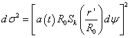
dσ² = [a(t)R₀S_k(r’/R₀)dψ]²

The current scale factor R₀ then plays the role of the curvature length, determining the distance over which the model is spatially Euclidean. Since the curvature radius would have to be constant in the Steady State model, the only possibility is that it is infinite and k = 0. Therefore, pure de Sitter space, in the original meaning of the phrase, is a Steady State universe. It has constant vacuum energy density, is of infinite age, and has no Big Bang. However, de Sitter space, in the original meaning of the phrase, has no matter.

If you add matter to a Steady State universe, it violates energy conservation since matter does not have the p = -ρc² equation of state that allows the density to remain constant. Therefore, Steady State models require the continuous creation of matter. Einstein’s equations are modified by adding a creation or C-field term to the energy-momentum tensor.

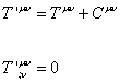
T’^uv = T^uv + C^uv

T’;_v^uv = 0

The effect of this extra term is to cancel the matter density and pressure, leaving just the overall effective form of the vacuum tensor, which is required to produce de Sitter space and the exponential expansion. This field is just added ad hoc, and had no physical motivation except for the problem it was supposed to solve. This Steady State model based on a modified version of general relativity to include a C-field was invented by William McCrea in 1951. In the middle of the 20th Century, the physics community was sharply divided between the Big Bang model and the Steady State model. The Big Bang proponents included George Gamow, Ralph Alpher, and Robert Herman. The Steady State proponents included Herman Bondi, Thomas Gold, and Fred Hoyle. Tempers flared as they argued passionately for their point of view. The Big Bang versus Steady State debate produced some remarkable displays of vitriol. British astronomer and Steady State proponent Fred Hoyle invented the name “Big Bang” as a derisive ridicule of the Big Bang model, and the name stuck.

This situation continued until Arno Penzias and Robert Wilson discovered the cosmic microwave background in 1964. This was interpreted as the faint afterglow of the intense radiation of a hot Big Bang predicted by Ralph Alpher and Robert Herman in 1949. Originally, the Universe was too hot for atomic nuclei and electrons to combine to form electrically neutral atoms. Then 379 ± 8 thousand years after the Big Bang, when the temperature cooled to 3000 K, the nuclei and electrons were moving slow enough to combine to form neutral atoms. Matter became electrically neutral, and matter decoupled from radiation. The photons set free by that decoupling are now being detected by us as cosmic background radiation. You could also think of it as blackbody radiation, like that which inspired Max Planck to come up with Planck’s constant, where in this case, the entire Universe is the cavity. The discovery of the cosmic microwave background provided overwhelming evidence for the Big Bang model. After that, the vast majority of physicists threw their support behind the Big Bang. Yet there remained a few staunch hold out who clung steadfast to the Steady State model. They tried to explain the cosmic microwave background by claiming it originated in interstellar dust. These claims were finally laid to rest in 1990, when it was demonstrated that the radiation was almost exactly Planckian in form. Other evidence for the Big Bang was that, following earlier work by Gamow, Alpher, and Herman in the 1940’s, theorists calculated the relative abundances of the elements hydrogen and helium that were produced in a hot Big Bang, and it was in good agreement with observation. Gamow originally claimed that all the elements were created in the Big Bang. In reality, only hydrogen and helium were created in the Big Bang, and the rest were created in stars.

You have to wonder why did some physicists so strongly prefer the Steady State model to the Big Bang model? Part of it is that they became wedded to a certain theory, and after advocating it so strongly, they became emotionally invested in it, and they were too proud to admit they were wrong, even in the face of overwhelming evidence. However, part of the reason is a justified desire to promote symmetry and invariance under transformations, which is one of the goals of physics. This is why some people today prefer eternal inflation. Physics is filled with symmetry groups, and systems that are invariant under transformations. With special relativity, you have Lorentz invariance. With the Standard Model, you have gauge invariance. You have all the symmetry groups of particle physics, such as SU(3) x SU(2) x U(1), SU(5), SO(10), SUSY, SO(32), E₈ x E₈, etc. In cosmology, this takes the form of homogeneity and isotropy. Homogeneity is a symmetry of translations, meaning the universe is invariant under translations. Isotropy is a symmetry of rotations, meaning the universe is invariant under rotations. However, if the universe existed for a finite length of time, then it is only homogeneous and isotropic in space but not in time. The universe is homogenous in space, meaning each point in space is basically the same, but it’s not homogenous in time, since each point in time during the history of the universe is not basically the same. The Universe is very different today than it was shortly after the Big Bang. The universe is isotropic in space, meaning if you look in any direction in space, you see basically the same thing, but it’s not isotropic in time, since if you look in any direction in time, you don’t see basically the same thing. If you look to the past, you see a finite length of time, 13.7 billion years, but if you look to the future, you see an infinite length of time ahead of you. Therefore, if the Universe existed for a finite length of time, it is homogeneous and isotropic in space but not in time. If the Universe existed for an infinite length of time, it is homogeneous in both space and time. In physics, you always want everything to be as symmetric as possible. That’s a common theme in physics. According to that, it would be better for the Universe to be homogeneous and isotropic in both space and time. This is called the perfect cosmological principle. This would have been a justified reason for someone to prefer the Steady State model to the Big Bang model, and is why some people today prefer eternal inflation.

Most physicists have no difficulty accepting new theories if they fit the data, and are the best explanation for what we observe. However, some people have a hard time changing their world view. Ernest Mach invented Mach’s Principle, but never accepted the reality of atoms. A whole generation of physicists who grew up on classical mechanics and electromagnetism never fully accepted relativity and quantum mechanics, despite the enormous success of those theories. Paul A. M. Dirac invented the Dirac equation, but never completely gave up the old classical view of particles and fields being two separate things. Similarly, many physicists who their whole lives assumed the Universe existed forever had a hard time accepting the Big Bang model, despite the mounting evidence. To go from the Steady State model to the Big Bang model involves radically changing your world view, and this is difficult for some people. Most physicists are willing to change their theories when confronted with new evidence. However, there are always a few people who just become wedded to a certain theory, and they cling to it even in the face of overwhelming evidence. In the case of the Big Bang, some people especially had difficulty accepting the idea of an initial singularity at t = 0, where there is no such thing as before that. The idea of a beginning of time itself, where there is no such thing as before that, is obviously outside our daily experience, and so it’s hard to imagine what that would be like. That’s not reason to reject it. Relativity and quantum mechanics are also very different from our daily experience, and many physicists initially had a hard time accepting those theories. Sometimes, a major change in our view of the Universe can only be accepted throughout the entire physics community when the older generation is replaced by the younger generation.

Inflationary cosmology was first suggested by Starobinsky, and was developed later by Andrei Linde and Alan Guth in 1981 to explain the horizon, flatness, and monopole problems. Inflation assumes an enormously large amount of expansion at the beginning of the universe. Extremely tiny regions on the planck scale are blown up to be larger than the observable universe. The inhomogeneities of the cosmic microwave background, as well as in the matter distribution, which gave rise to galaxies, originally began as quantum fluctuations. Now, you could imagine that this enormous expansion only took place at the beginning of the universe. Obviously, it’s not going on around us now. However, different parts of the universe could have different values of the scalar inflaton field that drives inflation. Therefore, some other part of the universe that is casually disconnected from us could be undergoing inflation. You could imagine that inflation ended within our observable universe but will always be going on in some parts of the universe, although in other parts it will settle down to a much lower rate of expansion, as in our part. Once you have that, there is no reason why the inflation that created our observable universe had to have taken place right after the Big Bang. It could have taken place any length of time after the Big Bang. You then have to differentiate between the effective local Big Bang, meaning when inflation ended within our part of the universe, which created our observable universe, and the original fundamental Big Bang, which was the origin of the entire universe. The local Big Bang did not necessarily take place right after the original Big Bang. There could have been 10¹⁰⁰ years between the original fundamental Big Bang, meaning the real origin of the entire universe, and our local Big Bang, meaning what we observe to be the Big Bang, which created our observable universe.

Once you say that, there is no reason not to take the theory to its logical conclusion, and say that there was no original fundamental Big Bang at all. You could just say that time extends infinitely backwards without beginning. Of course, there was what we normally call the Big Bang, which is the explanation for the redshifts of the galaxies, the cosmic microwave background, the isotropy of the cosmic microwave background to one part in 10⁵, etc. However, with inflation, it is no longer necessary that the Big Bang corresponds to a fundamental beginning of time itself. There could have been a beginning of time, but it’s equally possible that time extends infinitely backwards without beginning. This is almost like resurrecting the Steady State model. Alan Guth, who invented inflation in 1981, holds the view that there was a fundamental beginning of time. Russian cosmologist Andrei Linde advocates the view that time extends infinitely backwards without beginning. Andrei Linde was originally Soviet in addition to Russian, and now he’s American in addition to Russian. His theory that inflation has been going on for an infinite length of time is called eternal inflation. It has the advantage that the entire universe is homogeneous and isotropic in both space and time. Despite that, the vast majority of cosmologists share Alan Guth’s view that there was an original fundamental Big Bang, and Andrei Linde represents a small minority. The reason is similar to what I said earlier about followers of the Steady State model. The current generation of cosmologists grew up on the Big Bang, and the assumption there was a beginning of time. That’s what they were taught in school. Therefore, they feel that is much more logical. They’re not going to change their world view without a reason. Today, there is no observational evidence that can distinguish between normal inflation and eternal inflation, and not much reason to favor one over the other.

I will now explain Alan Guth’s model of inflation in more detail. I assume the reader has read my paper on the Standard Model. You might also want to read the section on grand unified theories in my paper Beyond The Standard Model. In quantum field theory, quantum fields produce an energy density that acts like a cosmological constant. In particle physics, especially extensions of the Standard Model, you have various scalar fields, such as Higgs fields, that could serve as the inflaton driving inflation, where they roll down a potential similar to how they do in the Higgs mechanism. The Lagrangian for a scalar field is kinetic minus potential energy.

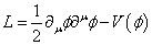
L = ½ [partial derivative]_u [phi] [partial derivative]^u [phi] – V([phi])

For instance, V(φ) could take the following form

V(φ) = ½ m²φ²

Noether’s theorem gives the energy momentum tensor as

T^uv = [partial derivative]^u[phi][partial derivative]^v[phi] – g^uvL

From this, you get the following energy density and pressure

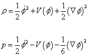
[rho] = ½ [phi dot]² + V([phi]) + ½ ([nabla][phi])²

p = ½ [phi dot]² – V([phi]) – 1/6 ([nabla][phi])²

If the field is constant both in space and time, then the equation of state is p = -ρ, which is what you need for it to act as a cosmological constant.

If φ is a complex Higgs field, you then get the symmetry breaking Mexican hat potential of the Higgs mechanism.

V(φ) = -μ² |φ|² + λ|φ|⁴

At the classical level, this says that |φ| will be located at the potential minimum. This gives the vacuum expectation value

< 0 | φ | 0>

However, this does not include the fluctuations that arise in thermal equilibrium. In classical systems, the non-zero temperature that a system of fixed volume will minimize is not the potential energy but the Helmholtz free energy, F = V – TS, where S is the entropy. The effect of thermal interaction is to add an interaction term to the Lagrangian.

L_int(φ, ψ)

Where ψ is a thermally fluctuating field that corresponds to the heat bath. You would expect L_int to have a quadratic dependence on | φ | around the origin.

L_int ∝ | φ |²

Otherwise, you would have to explain why the second derivative either vanishes or diverges. The coefficient of proportionality will be the square of an effective mass that depends on the thermal fluctuations in ψ. On dimensional grounds, the coefficient must be proportional to T².

Therefore, you have to minimize the following temperature dependent effective potential.

V_eff(φ, T) = V(φ, 0) + aT²|φ|²

The effect of this on the symmetry breaking potential depends on the form of the zero temperature V(φ). If the function is of the simple Higgs form

V = -μ² + λφ⁴

then the temperature dependent part modifies the effective value of μ².

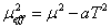
μ_eff² = μ² – aT²

At very high temperatures, the potential will be parabolic, with a minimum at |φ| = 0. Below the critical temperature

T_c = μ/[squareroot of a]

The ground state is at

|φ| = [squareroot of (μ_eff²/2λ)]

and you have broken symmetry. At any given time, there is only a single minimum, so this is a second order phase transition.

You could also have the following more complicated potential.

V_eff(φ T) = λ|φ|⁴ – b|φ|³ + aT²|φ|²

which has two critical temperatures. At very high temperatures, the potential will have a parabolic minimum at | φ | = 0. At T₁, there is a second minimum in V_eff at | φ | ≠ 0. This will be the global minimum for some T₂ < T₁. For T < T₂, the state at | φ | = 0 will be what is called a false vacuum, whereas the global minimum is called the true vacuum.

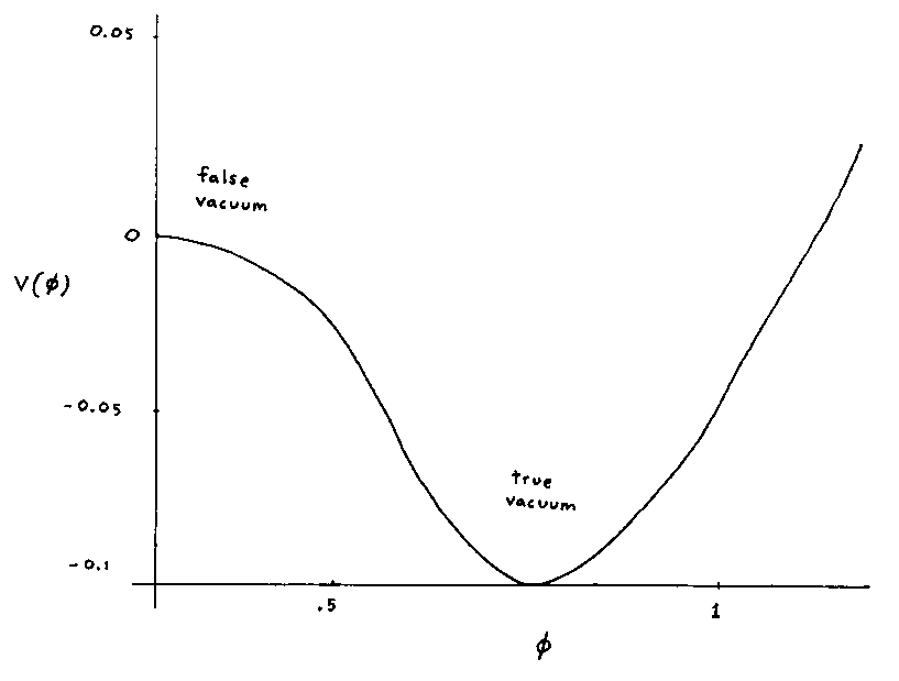
With this potential, the second minimum at φ = 0 always exists, so there is a potential preventing a transition to the false vacuum. This can be overcome by adding a small

-μ² |φ|²

component to the potential, so that there will a third critical temperature at which the curvature around the origin chances sign. Also, if the barrier is small enough, there will be quantum tunneling between the false and true vacuum.

The universe is no longer trapped in the false vacuum and can make a first order phase transition to the true vacuum. There will be an energy density difference between the two vacuum states.

ΔV = μ⁴/2λ

If you say that the zero of the energy is such that V = 0 in the true vacuum, this means that the false vacuum state acts as an effective cosmological constant. There must be an energy density of m⁴ in natural units, where m is the energy at which the phase transition occurs. In grand unified theories, m = 10¹⁶ GeV, so then

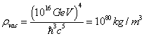
ρ_vac = (10¹⁶ GeV)⁴/[h bar]³c⁵ = 10⁸⁰ kg/m³

Therefore, there is an enormous amount of vacuum energy in grand unified theories, up until GUT symmetry breaking, after which it will stop. Therefore, grand unified theories predict an enormous amount of expansion of the universe at the very beginning of the universe, which is exactly the premise of inflationary cosmology.

The enormous amount of vacuum energy in models with GUT-scale symmetry breaking was a major motivation for inflation as originally envisioned by Alan Guth. The phase transition from false to true vacuum both terminates inflation, and also reheats the universe to the GUT temperature, allowing the possibility that GUT-based reactions that violate baryon number conservation can generate the observed matter-antimatter asymmetry. Since the transition is of first order, this is called first order inflation. However, while the final theory of inflationary cosmology will have the basic elements of vacuum-driven expansion, fluctuation generation, and reheating, it now appears that the final theory will have to be much more complicated than Alan Guth’s original theory.

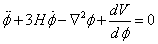
[phi double dot] + 3H[phi dot] – [nabla]²[phi] + dV/d[phi] = 0

In order to solve it, you have to make the slow roll approximation

| [phi double dot] |

is negligible compared to

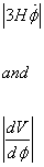
| 3H[phi dot] |

and

| dV/d[phi] |

The vacuum equation of state only holds if φ changes slowly both spatially and temporally. Let’s say you have temporal and spatial scales t and x for the scalar fields. The conditions for the inflation are that the negative pressure equation of state from V(φ) must dominate the normal pressure effects of time and space derivatives.

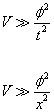
V >> φ²/t²

V >> φ²/x²

Therefore

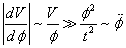
| dV/dφ | ~ V/φ >> φ/t² ~ [φ double dot]

The [φ double dot] term can be neglected in the equation of motion which then takes the slow-rolling form for homogenous fields.

3H[φ dot] = -dV/dφ

The condition

V >> [φ dot]²

can now be rewritten using the show-roll relation as

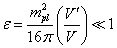
ε = m_pl²/16π (V’/V) << 1

Also, you can differentiate this expression to get the criterion

V’’ << V’/m_pl

Ultimately, you get

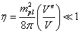
η = m_pl²/8π (V’’/V) << 1

The potential must be flat in the sense of having small derivatives if the field is going to roll slowly enough for inflation to be possible. If V is large enough for inflation to start in the first place, inhomogeneities rapidly become negligible. This stretching of field gradients as you increase the cosmological horizon beyond the value predicted in classical cosmology solves the monopole problem. Monopoles are point-like topological defects that arise at the GUT scale. If the horizon can be made much larger than the classical one at the end of inflation, the GUT fields then have to be aligned over a vast scale, so that topological defect formation would be extremely rare within our observable universe.

Next, I will try to illustrate the expansion and/or contraction of the universe in a variety of cosmological models, many of which have already been ruled out. You could imagine that the vertical axis is time, the horizontal axis is space, and the distance between the two vertical lines at any given time represents the volume of an arbitrary volume of space, which could be the entire universe for a closed finite universe. This is just to give a vague qualitative sense of a couple of models. The arrows on the side indicate whether time extends infinitely or not into the past or future. The small white circle is a singularity. With inflation, I just try to convey the general idea that as the universe is expanding, little pieces can suddenly expand to enormous size.

1. Steady State

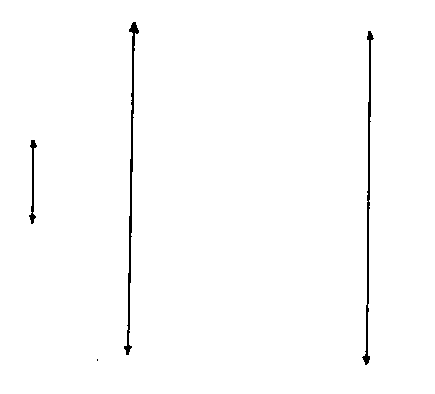
2. Big Bang, open or flat

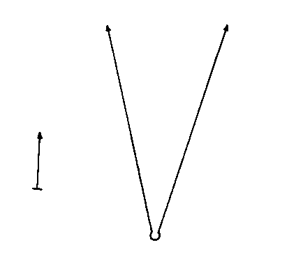
3. Big Bang, closed

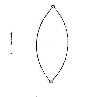
4. Inflation, with original fundamental Big Bang

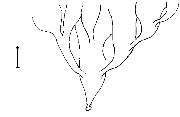
5. Eternal Inflation

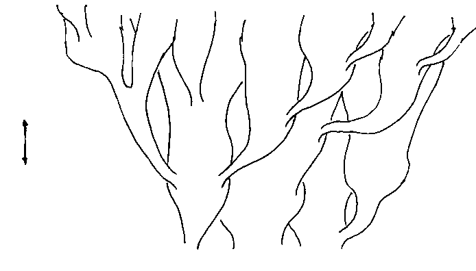
6. Ekpyrotic Universe

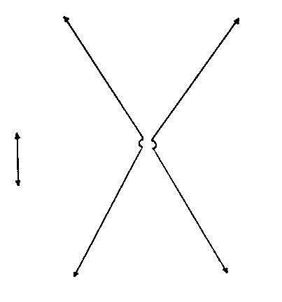
7. Cyclical Cosmology

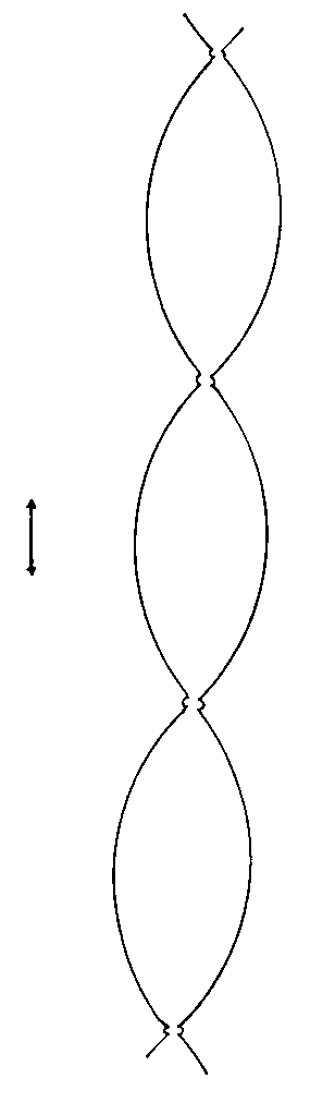
8. Cyclical Cosmology with original fundamental Big Bang

9. Eternal Contraction with Big Crunch

10. Bounce Cosmology

11. Loitering Cosmology

In the above list, the first one and the last three have already been ruled out. Inflation with a Big Bang is the most popular among cosmologists, and eternal inflation is the second most popular. Some prefer eternal inflation because it doesn’t have a Big Bang singularity. However, a singularity at the very beginning of the universe is not near as much a problem as a singularity in the middle of the history of the universe, which is what you have with the ekpyrotic and cyclical models. In these models, the universe existed before the singularity, and then it has to pass through a singularity afterwards. This is a serious problem for these theories at a fundamental theoretical level. In cyclical cosmology, the universe has to pass through a singularity an infinite number of times. Despite this, there are a few cosmologists who support the cyclical model. Originally inspired by Hinduism, the cyclical model was mentioned by both Carl Sagan and Star Trek.

A recent theory derived from superstring theory is brane world cosmology, which I describe at the end of my paper Beyond The Standard Model, as well as my short paper Brane World Cosmology. In this model, our universe is a D3-brane in higher dimensional space. The old cyclical model has been recast in the brane world scenario. They claim that there are two branes that attract each other, bounce off each other, or possibly pass through each other, and then attract each other again. Each collision is experienced as a Big Crunch/Big Bang on the branes. However, that’s still a form of singularity. This latest incarnation of cyclical cosmology does nothing about the problem of the universe having to pass through an infinite number of singularities.

The Universe contains luminous matter, such as stars, which makes up Ω_l = 0.05. In addition, you have nonluminous baryonic matter which makes up Ω_b = 0.047 ± 0.006. In addition, you have nonbaryonic dark matter, which gives you a total matter contribution of Ω_m = 0.29 ± 0.07. In addition, you have vacuum energy, sometimes called dark energy, which gives a contribution of Ω_Λ = 0.7, and radiation which contributes Ω_r = 10^-5. Now, how do we know how much all these things contribute, such as how much nonluminous baryonic matter there is, how much nonbaryonic matter there is, etc? Luminous matter, mostly stars, is the easiest to detect just by looking at the sky with a telescope that detects either visible light or other parts of the electromagnetic spectrum. This is normally done in galaxy surveys. We can calculate the amount of nonluminous baryonic matter in the Universe by looking at the Lyman alpha forests of interstellar and intergalactic hydrogen clouds. The Lyman series is the series of energies required to excite an electron in hydrogen from its lowest energy state to a higher state. A hydrogen atom with its electron in the lowest energy configuration is hit by a photon, and the electron is boosted to the second lowest energy level. The energy levels are given by E_n = -13.6 eV/n². The energy difference between the lowest level, n = 1, and the second lowest level, n = 2, corresponds to a photon with a wavelength of 1216 angstroms, where one angstrom = 10^-10 meters. You also have the reverse process where the electron goes from the n = 2 energy level to the ground state, and releases a photon with a wavelength of 1216 angstroms.

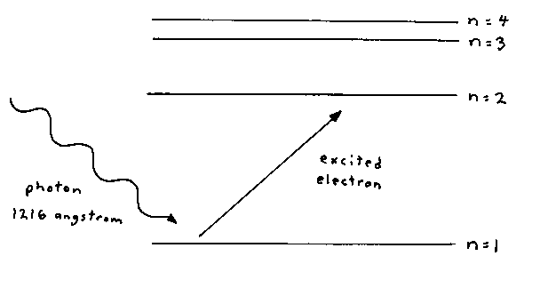
If you shine light with a wavelength of 1216 angstroms on a cloud of hydrogen atoms in their ground state, the atoms will absorb the light, and the electrons will be boosted to the next highest energy level. The more neutral hydrogen atoms in their ground state, the more light they will absorb. If you look at the light you receive, intensity as a function of wavelength, you will see a dip in the intensity at 1216 angstroms that depends on the amount of neutral hydrogen present. The amount of light absorbed, or optical depth, is proportional to the probability that the hydrogen will absorb the photon, which is the cross section, times the number of hydrogen atoms along its path. In cosmology, the hydrogen is in interstellar or intergalactic gas clouds, and the light source is quasars.

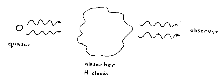
Neutral hydrogen atoms will interact with whatever light has been redshifted to a wavelength of 1216 angstroms when it reaches them. The rest of the light will keep traveling to us. From seeing how 1216 angstrom light is absorbed throughout the sky, you can calculate how much hydrogen is in the Universe.

The quasar shines with a certain spectrum or distribution of energies. Gas around the quasar both emits and absorbs photons. With the presence of neutral hydrogen, including that near the quasar, the emitted flux is depleted for certain wavelengths, indicating the absorption by this intervening neutral hydrogen. Since the 1216 angstrom wavelength is preferentially absorbed, we know that at the location at which the photon was absorbed, it probably had a wavelength of 1216 angstroms. Its wavelength was redshifted by the expansion of the Universe from what it was when it was emitted by the quasar, and if it had continued to travel to us, it would have continued to redshift beyond the 1216 angstroms it had at the absorber. Thus you see a dip in the flux at the wavelength corresponding to the 1216 angstroms the photon would have had if it had reached us. Since we can calculate how the Universe is expanding, we can tell where the photons were absorbed in relation to us. Therefore, you can use the absorption map to plot the positions of the intervening hydrogen clouds between us and the quasar.

It is common to see a series of absorption lines called the Lyman alpha forest. Systems which are more dense, called Lyman limit systems, are so thick that radiation doesn’t get into their interior. Inside these clouds, there is some neutral hydrogen remaining, screened by the outer cloud layers. If the clouds are very thick, there is instead a wide trough in the absorption. This is called a damped Lyman alpha system. Absorption lines usually aren’t at one fixed wavelength, but over a range of wavelengths, with a width and intensity determined by the lifetime of the excited n = 2 hydrogen state. These damped Lyman have enough absorption to show details of the line shape such as that determined by the excited state. Lyman alpha forest systems have 10¹⁴ atoms per centimeter. Lyman limit systems have 10¹⁷ atoms per square centimeter. Damped Lyman alpha systems have 10²⁰ atoms per square centimeter.

Lyman alpha systems can also be used to measure the amount of deuterium in the Universe. The higher the baryon density in the early universe, the more deuterium would be converted into helium. The lower the baryon density in the early universe, the less deuterium would be converted into helium. Therefore, the more deuterium we detect today, the lower the baryon density of the universe. The less deuterium we detect today, the higher the baryon density of the universe. We detect large amounts of deuterium, which means we have a low baryon density. Also, astrophysical processes are a net destroyer of deuterium, which means that you originally had even more deuterium, which would mean an even lower baryon density. From this, we calculate the amount of baryonic matter in the Universe.

How do you determine the amount of dark matter in the Universe? As far as we know, it can only interact gravitationally, so it can only be detected through gravitational interactions. You can look at the rotation of galaxies, or look at bound systems of galaxies, and calculate how much additional mass would have to be present to keep the system bound. The main way of detecting dark matter is through gravitational lensing. According to general relativity, the presence of matter or energy density will curve spacetime, and the path of light will also be deflected. The amount it is deflected tells you the amount of intervening matter. This is called gravitational lensing. The mass that bends the light is called the lens. In fact, this is what provided proof for general relativity, during the 1919 eclipse. Usually, you don’t have to actually solve the general relativistic equations of motion for the coupled spacetime and matter, because the bending of spacetime by matter is small. The matter curving space is moving slowly relative to c, and the gravitational potential φ induced by matter obeys

| φ | /c² << 1

Here is light from a distant source being deflected by an intervening mass.

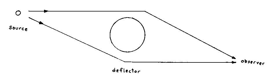
The light can be any type of radiation. Light rays that would otherwise not reach the observer are bent from their paths and towards the observers. Light can also be bent away from the observer. Gravitational lensing is divided into three types, which are strong lensing, weak lensing, and microlensing, based on the amount of deflection. Strong lensing is the most extreme bending of light, and is when the lens is very massive, and the source is close to it. In this case, light can take different paths to the observer, and more than one image of the source will appear. The first example of a double image was that of a quasar in 1979. The number of lenses discovered can be used to estimate the volume of space back to the sources. The volume depends on cosmological parameters, especially the cosmological constant. If the brightness of the source varies with time, the multiple images will also vary with time. However, the light doesn’t travel the same distance to each image, due to the curving of space. Therefore, there will be time delays for the changes in each image. These time delays can be used to calculate Hubble’s constant. In some rare cases, the alignment of the source and the lens will be such that light will be deflected to the observer in a ring called Einstein’s ring. More often than a perfect ring, the source will form an arc. It takes a lot of mass to form an arc, so the properties of arcs, such as number, size, and shape, can be used to study very massive objects, such as clusters. Given a set of images, you can try to reconstruct the lens mass distribution.

Weak lensing is when the lens is not strong enough to create multiple images, arcs, or a ring, but instead the source is distorted by being stretched, called sheer, and/or magnified, called convergence. If all the sources are well known in size and shape, you could just use sheer and convergence to deduce the properties of the lens. However, usually you don’t know the intrinsic properties of the sources, and instead only have knowledge of average properties. The statistics of sources can then be used to get information about the lens. If there is a distribution of galaxies far enough away to serve as sources, then clusters nearby can be weighted, meaning have their masses measured, using lensing. The statistical properties of large scale structure can also be measured by weak lensing, because the matter will produce sheer and convergence in distant sources. Weak lensing is used to compliment measures of the distribution of luminous matter, such as galaxy surveys. Lensing measures all mass, both luminous matter and dark matter. Microlensing is when the lensing of an object is so small that it just makes the image appear brighter. The additional light bent towards the observer means that the source appears brighter. This can be good when you are trying to view an object that would otherwise be too dim to see. However, it’s more often a nuisance, such as when you trying to measure the distance to an object, and thus need its apparent brightness, or when you are trying to measure all objects brighter than a certain amount in a certain region, and microlensing brings additional objects into the sample you don’t want. Gravitational lensing measures all mass, including dark matter, and thus is our main away of measuring the amount of nonbaryonic matter in the Universe.

It was always assumed that there was some nonluminious matter in the Universe. For instance, planets would count as nonluminous. However, the mass of all the planets in the Solar System put together is less than one percent the mass of the Sun. Therefore, it was assumed that nonluminous matter was negligible. Then in the 1930’s, Zwicky and Smith both examined two nearby clusters of galaxies, the Virgo Cluster and the Coma Cluster. They studied the galaxies making up the clusters, and their velocities, and determined that the velocities of the galaxies was 10 – 100 times too large. The velocities indicate the total mass in two ways. First of all, the more mass in the cluster, the greater the gravitational forces acting on each galaxy, which accelerates the galaxies to higher velocities. Second of all, if the velocity of a given galaxy is too large, the galaxy will be able to break free of the gravitational pull of the cluster. If the galaxy’s velocity is larger than the escape velocity, the galaxy will leave the cluster. By assuming that all galaxies in a cluster have velocities less than the escape velocity, you can estimate the total mass. This was the first suggestion of significant amounts of nonluminous matter in the Universe. However, it was inconclusive. Even though the velocities are large, the clusters of galaxies are so stupendously large, that the galaxies appear to move in slow motion. So, it’s as if we only get to see one frame of a movie. Maybe a galaxy with high velocity really is leaving the cluster. Maybe it was never part of the cluster in the first place, and was just passing through. Maybe some of the galaxies that you are including in the cluster are just foreground galaxies in the line of sight.

In the 1970’s, Rubin, Freeman, Peebles, and others started measuring the rotation curves of galaxies. According to Kepler’s Laws, an orbiting body should move slower the farther it is from the axis of rotation, which is the center mass it’s orbiting. For instance, in the Solar System, Pluto moves much slower than Mercury. However, this is not what they found for galaxies. With spiral galaxies, the velocities of the stars did not decrease as you got farther from the center of the galaxy. The Milky Way rotates once every ¼ billion years, so they could only detect the velocities by the Doppler effect. As you look at spiral galaxies, the velocities of the stars remain high all the way out to the edge. This strongly suggests that what you think is the edge of the galaxy is only the edge of the luminous matter in the galaxy, and the rest of the galaxy, which is dark matter, extends for a much greater distance away from the center of the galaxy. By finding the rotation velocities along a galaxy, you can weigh the mass of the galaxy inside the orbit. This was the first strong evidence for dark matter. Later, you had evidence from gravitational lensing. Also, inflationary cosmology predicted the universe was flat, and the amount of luminous matter was not enough to flatten the universe. We now know that even the dark matter is not enough to flatten the universe, and you need dark energy.

Today, our view of the Universe according to cosmology is totally consistent within itself, and with observation, such as the recent WMAP data, other CMB data, and the supernovae Ia data. However, one very obvious gap in our knowledge is that even though we can talk about dark matter, and include it in our equations, we don’t know what it actually is. This is probably the most obvious unanswered question in physics today. Now at first it was hoped that dark matter could be something normal such as planets, Jupiters, brown dwarves, or white dwarves. Planets could only contribute a maximum of Ω = 0.005. Jupiters are Jupiter-like planets. Brown dwarves are failed stars not large enough to ignite, larger than Jupiter but smaller than the Sun. White dwarves are the final stage of stars like the Sun. However, all of these things are made of baryons. We can measure the amount of baryonic matter in the Universe, and it’s much less than what we measure the dark matter to be. That means dark matter must be nonbaryonic matter.

Here, I list the primary candidates for nonbaryonic dark matter. They are listed in order of how likely they are, or how mainstream the theory is. Since these are mostly derived from particle physics, you should read my papers The Standard Model, and Beyond The Standard Model for more information.

1. Neutrinos – These are Standard Model leptons. Since neutrino oscillation has proved that neutrinos have mass, they were an obvious candidate for dark matter. However, it was determined that the neutrino masses are so small that they can only account for a small percentage of the dark matter. Today, we assume that a small percentage of the dark matter is due to neutrinos, and we’re trying to explain the rest of it.

2. Supersymmetric Particles – We invented supersymmetry to explain the hierarchy problem, and the theory doubles the number of particles. According to the minimal supersymmetric standard model, the lightest supersymmetric particle, or LSP, should be stable, and could account for dark mater. It’s usually called a neutalino. These are considered weakly interacting massive particles, or WIMP’s.

3. Axions – These are Goldstone bosons formed by Peccei-Quinn symmetry breaking.

4. Primordial Back Holes – According to some theories, large numbers of tiny black holes could be left over from the Big Bang.

5. Cosmic Strings – This is a one dimensional topological defect.

6. Strangelets – Some theories claim you can have stable particles containing strange quarks.

7. Quark Nuggets – Some theories claim you could have macroscopic amounts of quark matter.

8. Fermi Balls – Symmetry breaking creates domains in the early universe. These bubbles of false vacuum would shrink down but might stop at a non-zero size if they contain fermions. Fermi balls are non-topological solitons.

9. Q-balls – This is another type of non-topological soliton.

10. Mirror Fermions – Some theories designed to explain why the Standard Model is chiral predict mirror fermions.

11. Chaplygin Gas – This is an entity with an exotic equation of state that could explain both dark matter and dark energy.

12. Quartessence – A version of quintessence that claims to explain not only the dark energy but the dark matter also.

There are tons of other suggestions that I won’t bother to mention. Physicists certainly don’t lack imagination when it comes to thinking up new candidates for dark matter. The proliferation of suggestions indicates the lack of evidence for what it actually is.

There used to be an alternative to dark matter as an explanation for galactic rotations called MOND. It was observed that the star velocities do not decrease as you go out to the edge of the galaxy, as they should according to Newtonian mechanics. The common explanation was that there is matter in the galaxy that extends far beyond what we can see. An alternative explanation is that Newtonian mechanics has to be modified at large distances. This is called Modified Newtonian Mechanics, or MOND, and was invented by Milgrom in 1983. It involves just adding terms to the equations to make the predictions fit the rotation curves of galaxies. The fact it fits is not surprising since it was designed to do just that. The main problem with MOND at the theoretical level was that it was totally ad hoc and not motivated by underlying physics. As time went on, there was more and more observational evidence for dark matter until the evidence was overwhelming. Dark matter basically won that debate. In physics, you try to choose the simplest explanation. Most people felt the simplest explanation was dark matter, and MOND was too radical. The few supporters of MOND sincerely believed that MOND was the simpler explanation, and that dark matter was too radical.

The existence of the cosmic microwave background radiation was first predicted by George Gamow in 1948, and by Ralph Alpher and Robert Herman in 1949. It was first detected by Arno Penzias and Robert Wilson in 1964 at the Bell Telephone Laboratories in Murray Hill, New Jersey. They had no clue what it was. They thought it was just a source of excess noise in the microwave radio receiver they were building. They went so far as to clean the pigeon shit out of the microwave antenna to try to get rid of it. Coincidentally, at that same time, researchers led by Robert Dicke at the nearby Princeton University were devising an experiment to try to detect the cosmic microwave background. When they first heard about the problems Penzias and Wilson were having with the background static, they instantly recognized what it was. They were enthusiastic that the cosmic microwave background had been found. There was then a pair of papers in Physical Review. One was by Penzias and Wilson describing their observations. The other was by Dicke, Peebles, and Wilkinson declaring that this was in fact the long sought cosmic microwave background. Later, Penzias and Wilson received the 1979 Nobel prize in physics.

Since then, there have been numerous experiments designed to study the cosmic microwave background, which is isotropic to one part in 10⁵, but does have anisotropies which reveal a great deal about the Universe. Most recent experiments were intended to probe the anisotropies in the CMB. It turns out that the temperature fluctuations in the CMB are a very close match to what is theoretically predicted by inflationary cosmology. The COBE satellite was launched in 1989, and carried three instruments. The Diffuse Infrared Background Experiment searched for cosmic infrafred background radiation. The Differential Microwave Radiometer measured the cosmic microwave radiation. The Far Infrared Absolute Spectraphotometer compared the spectrum of the cosmic microwave background radiation with a perfect blackbody. BOOMERANG was a balloon based experiment that floated around Antarctica for ten days in 1998. The name was a pun since they released it, it went around in a circle, and then it came back to where they released it. Here, I’ll list the major experiments. Satellite CMB experiments include WMAP, COBE, Planck, and DIMES. Balloon-based experiments include BOOMERANG, MAXIMA, FIRS, ARGO, MAX, QMAP, and many others. Ground-based experiments include DASI, COBRA, VSA, CBI, IAC, White, Dish, CAT, OVRO, ACBAR, and many others. One of the people on Robert Dicke’s team in 1964 was Dave Wilkinson who later spearheaded a project to create a probe called the Microwave Anisotropy Probe, or MAP. When Wilkinson died, it was renamed the Wilkinson Anisotropy Probe, or WMAP. In June 2001, a Delta rocket launched NASA’s 840 kg Microwave Anisotropy Probe on a journey that took it to the L2 Lagrange point, 1.5 million km antisunward from Earth. Then the probe began continuously mapping with unprecedented precision, the very small departures from the almost perfect isotropy of the cosmic background radiation, and the even fainter polarization caused by these anisotropies. The WMAP probe has given us far better cosmological data than we’ve ever had before.

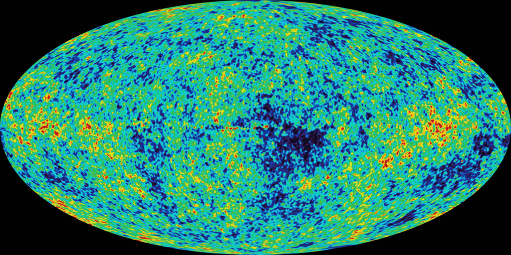
Some people hailed WMAP as the beginning of precision cosmology. Of course, people said the same thing about Galileo’s work. WMAP’s design was optimized to improve the calibration uncertainties of previous CMB probes by an order of magnitude. With its sensitivity and uninterrupted full sky coverage at five different microwave frequencies. WMAP measured the first acoustic peak in the CMB temperature anisotropy power spectrum with error bars smaller than the cosmic variance that randomizes the power spectrum seen by an observer at any given location in the Universe. The microkelvin hot and cold regions in the all sky map of the CMB from WMAP indicate local regions at the end of the plasma epoch that had mass densities very slightly higher or lower than the mean. The expansion and contraction of such density fluctuations are acoustic wave phenomena in the viscous elastic plasma fluid in which radiation pressure completes with gravitational contraction. The sound speed that limits how fast a hot or cold spot could have expanded in the plasma is about C/[squareroot of 3]. To compare the CMB observations with theory and extract the best-fit cosmological parameters, it is useful to obtain the angular power spectrum of temperature fluctuations by decomposing the celestial map of departures ΔT from the mean CMB temperature into a sum of spherical harmonics

Y_{l, m}(θ, φ)

Where l is lower case “L”, and is the multipole moment, and m is the azimuthal index.

Temperature fluctuations on the microwave sky can be expressed as a sum of spherical harmonics, similar to how music can be expressed as a sum of ordinary harmonics. A musical note is the sum of the fundamental, second harmonic, third harmonic, etc. The relative strengths of the harmonics determine the tone quality, which distinguishes a middle C played on a flute and a clarinet. The temperature map of the microwave sky is the sum of the spherical harmonics, or the power spectrum, and indicate the geometry of the Universe.

The fluctuation power at multipole l is then given by the mean square value of the expansion coefficients a_{l, m} averaged over the 2l + 1 values of the azimuthal index m. Since there is no preferred direction on the CMB sky, the distribution of power m varies randomly with the observer’s position in the Universe. Therefore, the cosmic variance is widest at small l. The only slight discrepancy in the WMAP data with the theoretical prediction is the slightly low quadrupole. The temperature fluctuation power for a given l measures the mean square temperature difference between points on the sky separated by an angle of order π/l. The harmonic sequence of distinct acoustic peaks is attributed to the abrupt beginning and end of the plasma epoch. The end catches different oscillation modes that happen to be maximally overdense or underdense at the instant CMB photons were set free. The positions and heights of the peaks constrain cosmological parameters. The l range of a CMB telescope is limited by its angular resolution. WMAP has an angular resolution of about 12 arcminutes so it can’t follow the power spectrum beyond l = 800. CBI and ACBAR are two ground-based microwave telescopes with finer angular resolution than WMAP. Here is the data from many different CMB experiments, plotting multipole versus temperature fluctuation.

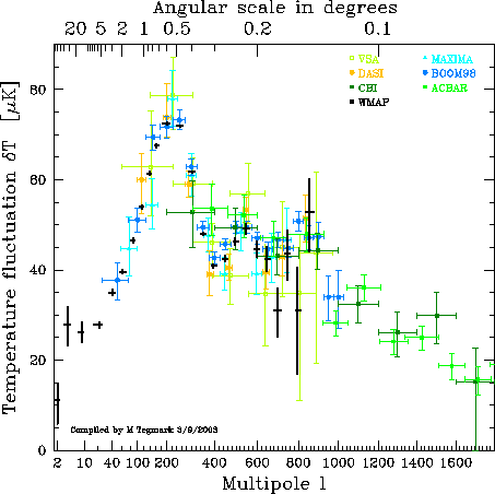
WMAP greatly increased of knowledge of several cosmological parameters, some of which are listed below.

Baryon Density

Ω_bh² = 0.024 ± 0.001

Matter Density

Ω_mh² = 0.14 ± 0.02

Hubble’s Constant

h = 0.72 ± 0.05

Amplitude

A = 0.9 ± 0.1

Optical Depth

τ = 0.166_{– 0.071}^{+ 0.076}

Spectral Index

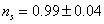
n_s = 0.99 ± 0.04

Amplitude of Galaxy Fluctuations

σ₈ = 0.9 ± 0.1

Characteristic Amplitude of Velocity Fluctuations

σ₈Ω_m^0.6 = 0.44 ± 0.10

Baryon Density/Critical Density

Ω_b = 0.047 ± 0.006

Matter Density/Critical Density

Ω_m = 0.29 ± 0.07

Age of the Universe

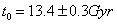
t₀ = 13.4 ± 0.3 Gyr

Redshift at Reionization

z_r = 17 ± 5

Redshift at Decoupling

z_dec = 1088_{– 2}^{+ 1}

Age of the Universe at Decoupling

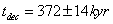
t_dec = 372 ± 14 kyr

Thickness of Surface at Last Scatter

Δz_dec = 194 ± 2

Duration of Last Scatter

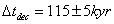
Δt_dec = 115 ± 5 kyr

Redshift at Matter/Radiation Equality

z_eq = 3454_{– 392}^{+ 385}

Sound Horizon at Decoupling

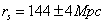
r_s = 144 ± 4 Mpc

Angular Diameter Distance to the Decoupling Surface

d_A = 13.7 ± 0.5 Cpc

Acoustic Angular Scale

l_A = 299 ± 2

Current Density of Baryons

n_b = (2.7 ± 0.1) x 10^-7 cm^-3

Baryon/Photon Ratio

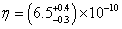
η = (6.5 _{– 0.3}^{+ 0.4}) x 10^-10

Next I will give a brief history of the Universe. As you go farther and farther back in time, the Universe gets more and more different than it is right now, so we understand progressively less as you go farther back in time. We are less sure of the entries in the beginning, and get more sure as you go on. Therefore, at some point you switch from “universe” to “Universe”. Also, we don’t even know whether the Universe existed for a finite or infinite length of time. For the purpose of this discussion, I’m assuming that the universe began in an initial singularity. If you look at the current expansion, and extrapolate backwards, you end up with a singularity, and so here I’m assuming that happened, although we don’t know if it did nor not. When I say singularity, I mean the singularity that would be there if you extrapolate all the way backwards. Also, the times that you are referring to can be labeled by length of time since the Big Bang, length of time ago, energy scale in eV, temperature in K, or redshift, where t is length of time since Big Bang, T is the temperature, and z is the redshift. In some regimes, it’s more appropriate to use one unit of measurement, and in other regimes, it’s more appropriate to use another. You will understand it better, if you have read my papers The Standard Model, and Beyond The Standard Model.

1. Singularity, t = 0, T = ∞, 13.7 ± 0.2 billion years ago

Initial singularity, origin of spacetime itself, the Big Bang

2. Planck Scale, t = 10^-42 seconds or the Planck time, T = 10¹⁹ GeV, T = 10³² K

Gravity is as strong as the other forces. All four forces are unified, and you have one force. Then gravity separates from the other forces but still has to be described by quantum gravity. You have quantum gravity effects at the Planck scale. In string theory and M-theory, all the dimensions begin as compactified. According to M-theory, the universe has 10 spatial dimensions which are all the same, and all small. Then due to the Brandenbeurger-Vafa mechanism, three of the spatial dimensions expand into the obvious ones we have today, leaving seven compactified. According to string theory, the details of the topology that the extra dimensions are compactified on, determines the vibration modes of the strings which determine what fundamental particles exist. Also, primordial black holes might be produced at this time.

3. Grand Unification Scale, T = 10¹⁶ GeV

Before now, there was no difference between the electroweak and the strong force. They were just one force. Since X and Y bosons are essentially massless compared to the energy scale, they are freely created, and thus quarks and leptons can be freely converted into each other. At the grand unification scale, the grand unified theory undergoes symmetry breaking. It probably undergoes several successive stages of symmetry breaking, as larger groups go through a cascade down to smaller groups. For instance, according to string theory, it could possibly go from E₈ x E₈ to E₆ x E₈ to SO(10) to SU(5) to the Standard Model U(1) x SU(2) x SU(3). Also, topological defects such as monopoles would be produced.

4. Inflation, t = 10^-36 seconds

At some point, inflation ends. It is probably after grand unification, so that topological defects formed by grand unified theory symmetry breaking, would be rare within our observable universe. The inflaton field rolls down to the bottom of its potential from false vacuum to true vacuum, and after that, inflation occurs at a much more leisurely pace.

5. Peccei-Quinn Symmetry Breaking

The Peccei-Quinn (PQ) symmetry breaking, as proposed in the Peccei-Quinn theory, is believed to have occurred spontaneously at high energies, likely during the early universe’s evolution, specifically around the time of inflation or shortly after. This breaking is thought to have given rise to the axion, a hypothetical particle that could solve the strong CP problem in particle physics. In 1977, Roberto Peccei and Helen Quinn proposed a new global U(1) symmetry, called the PQ symmetry, to address the strong CP problem in quantum chromodynamics (QCD).

6. Supersymmetry Breaking, T = 1 TeV = 1000 GeV, T = 10¹⁹ K

Before supersymmetry breaking, supersymmetry was an unbroken symmetry. Supersymmetric particles, such as squarks, sleptons, and bosinos, were as common as what we call normal particles, such as quarks, leptons, and bosons. After supersymmetry breaking, we are left with only normal particles, with the possible exception of the lightest supersymmetric particle.

7. Electroweak Phase Transition, t = 10^-11 seconds or 10 picoseconds, T = 100 – 200 GeV, T = 1 – 2 x 10¹⁵ K or 1 – 2 quadrillion K

Before this, there was no difference between the electromagnetic and weak force. They were just one force. When the temperature got low enough, there was symmetry breaking. You have the Higgs mechanism go into effect. Before that, you had a complex Higgs doublet, and the three massless intermediate vector bosons. Afterwards, you have the massive W⁺, W^–, and Z⁰, the massless photon, and a leftover Higgs. This is for the Standard Model Higgs particles. You also have a similar thing happen earlier with the Higgs fields associated with grand unification and supersymmetry.

8. QCD Phase Transition, t = 5 x 10^-5 seconds or 50 microseconds, T = 150 – 180 MeV, T = 1.7 x 10¹² – 2.1 x 10¹² K or 1.7 – 2.1 trillion K

This is also called QCD Confinement or the Quark-Hadron Transition. Before this, you had a sea of free quarks and gluons. After this, quarks are moving slow enough that they are confined to hadrons. Therefore, hadrons first come into existence. The strong force is weak at high energies, which is the same at short distances, and strong at low energies, which is the same as large distances. Therefore, normally quarks can never get out of hadrons. However, at high enough energies, the distinction between inside a hadron and outside a hadron disappears, and you have a quark-gluon plasma. Most people think the QCD phase transition is a first order transition, meaning heat is emitted as the transition happens, just as when water vapor condenses to form drops of liquid water. Therefore, the quark-gluon plasma would probably supercool until small bubbles of hadron phase formed. As these bubbles grew, latent heat would be emitted. This would reheat the quark-gluon plasma, limiting the speed at which the bubbles expanded. Heat would be dispersed by neutrino and acoustic waves. Some people call the creation of the first hadrons baryogenesis.

9. Annihilation of Pions, t = 10^-4 seconds or 100 microseconds, T = 100 MeV, T = 10¹² K or 1 trillion K

If you provide energy equivalent to a particular particle’s rest mass, you can create that particle. If the temperature is enormously high, then just the kinetic energy of the motions of the particles will be enough to create new particles. If the temperature is above a trillion Kelvin, then the kinetic energy will be enough to create pions which have a mass of about 100 MeV. Therefore, since the QCD phase transition, the universe was filled with pions, which were constantly being created to replenish those that annihilated. When the temperature dropped below a trillion Kelvin, pions were no longer being continuously created, and those that remained annihilated each other.

10. Decoupling of Neutrinos, t = 1 second, T = 1 MeV, T = 10¹⁰ K or 10 billion K

Neutrinos can easily zip through light-years of lead but the very early universe was so compressed and so dense that they couldn’t get very far, and interacted vigorously with other forms of matter. However, about one second after the Big Bang, the density of the universe decreased to about 400,000 times that of water, and neutrinos decoupled from other matter. Since these neutrinos were not reheated by nucleosynthesis, they should now be cooler than the cosmic microwave background radiation. They should be 2 Kelvin instead of 2.725 Kelvin. These primordial neutrinos should now fill the universe, but we can’t detect them because they move so slowly.

11. Annihilation of Electron-Positron Pairs, t = 10 seconds, T = 500 keV, T = 5 x 10⁹ K or 5 billion K

The rest mass of an electron is about 511 MeV, so it takes twice that much energy to create an electron-positron pair. If you multiply 511 MeV by Boltzmann’s constant, k = 1.38066 x 10^-23 J/K, you get about 5 billion Kelvin. That means that at this temperature, two particles colliding head on will often have enough kinetic energy to create an electron-positron pair. Therefore above this temperature a large number of electrons and positrons will be continuously created by just the collisions between particles. When the temperature drops below this, electrons and positrons will stop being created in such numbers, and most of those remaining will annihilate each other. Some people refer to this as leptogenesis.

12. Nucleosynthesis, t = 180 seconds, T = 100 keV, T = 10⁹ K or 1 billion K

At about this time, the temperature dropped to the point where a proton and neutron could stick together forming a deuterium nucleus. Then deuterium nuclei could bind together to create helium nuclei. This is called nucleosynthesis. This is responsible for the fact that before the first stars, the baryonic matter was 75% hydrogen and 25% helium.

13. Decay of Lone Neutrons, t = 1000 seconds, T = 50 keV, T = 5 x 10⁸ K or 500 million K

A lone neutron has a lifetime of 918 seconds, after which it will decay into a proton, electron, and antineutrino. Any neutrinos that are not bound in nuclei decay at this time.

14. End of Radiation-Dominated Era, t = 10,000 years, T = 1 eV, T = 12,000 K, z = 3454

Up until this point, the Universe was radiation-dominated. Here it makes the transition from radiation-dominated to matter-dominated. It remained matter-dominated until the present epoch when we have comparable contributions from the matter density and vacuum density. In the future, it will be vacuum-dominated. The end of the radiation-dominated era is when gravity began to amplify small fluctuations in the density of matter. This led to matter collapsing under gravity on various size scales to lead to stars, galaxies, and clusters of galaxies.

15. Recombination, t = 380,000 years, T = 3000 K, z = 1088

Before this, you had atomic nuclei and free electrons. After this, atomic nuclei and electrons are moving slow enough that they can bind to form atoms. Therefore, atoms first come into existence. In chemistry, when an atomic nucleus combines with electrons to form an atom, they call it “recombination”. However, in this case, they are combining for the first time. A better name would be “combination” instead of recombination, which is the official name. Before this, the Universe was filled with electrically charged plasma. After this, it was filled with neutral hydrogen. Plasma absorbs light at all frequencies, while electrically neutral gases tend to be transparent except for certain frequency bands. Therefore, recombination was the first time that photons could travel for long distances without being absorbed. The first photons that were set free to travel are now being detected by us as the cosmic microwave background radiation.

16. Drag Epoch, t = 400,000 years, T = 2900 K, z = 1060

The Drag Epoch is the specific moment in the early universe when baryonic matter (protons and electrons) completely decoupled from the radiation field of photons. Before this event, intense radiation pressure dragged normal matter along with it, preventing gravity from pooling the atoms into structures. Once the drag epoch ended, matter was freed from this “photon drag,” allowing it to gravitationally collapse and eventually form the first stars and galaxies. Because photons vastly outnumbered baryons (by roughly a billion to one), photons stopped interacting with matter first. However, even a tiny fraction of remaining scattering events was enough for the massive sea of photons to continue exerting a “drag” on the much smaller population of baryons.

17. Cosmic Dawn, t = 100 – 200 million years, T = 57 – 85, z = 20 – 30

Cosmic Dawn, the period when the first stars and galaxies began to form, is estimated to have occurred between 250 and 350 million years after the Big Bang. Cosmic Dawn refers to the period in the universe’s history, roughly 50 to 1 billion years after the Big Bang, when the first stars and galaxies began to form. This era marks the transition from a universe dominated by neutral hydrogen to one with luminous structures and is a key period for understanding the universe’s evolution. Here I am talking about the beginning of Cosmic Dawn. The entire length of Cosmic Dawn could be said to be 100 – 550 million years after the Big Bang. It overlaps with, and caused, Reionization

18. Reionization, t = 200 million years, T = 50 K, z = 17 ± 5

This is when the neutral hydrogen, which had cooled after the Big Bang, became hot and ionized again. This was probably caused by the first stars, so this would mean the first stars were formed about 200 million years after the Big Bang. Also during this time, you have the formation of large scale structure due to the clumping of matter under gravity. We believe that galaxy formation is caused by gravitational clumping that was seeded by dark matter. We can detect a rough correlation between anisotropies in the CMB and large scale structure.

19. Cosmic Noon – 2 – 3 billion years after the Big Bang, 11 – 10 billion years ago, z = 1 – 3

Cosmic Noon refers to a period in the universe’s history, roughly 10 to 11 billion years ago, when the rate of star formation and black hole growth reached its peak. During this epoch, galaxies were undergoing intense periods of star formation, and supermassive black holes were rapidly growing and actively reshaping their surroundings. Cosmic Noon represents the time when galaxies were forming stars at their highest rate. This era is crucial for understanding how galaxies assembled their stellar mass and evolved. It was also a time of intense black hole activity, with supermassive black holes rapidly accreting matter and growing in size. The intense star formation and black hole activity during Cosmic Noon played a significant role in shaping the properties of galaxies as we see them today.

20. Present Era, t = 13.7 x 10⁹ years or 13.7 billion years, T = 2.725 K, z = 0

This is the present. The Universe is 13.7 ± 0.2 years old. The cosmic microwave background now has a temperature of 2.725 K. During the present era, Ω_m = 0.3 and Ω_Λ = 0.7. Therefore, during the present era, the matter density is becoming of the same order as the vacuum density. The fact that this happens to be happening during the time we are is called the cosmic coincidence problem.

Let’s say you are watching ice freeze on a pond in the middle of winter. The ice does not form on the surface everywhere at once, and it doesn’t grow from one single point. Instead, the water begins to freeze in many places independently, and the growing plates of ice join up in a random fashion leaving zig-zag boundaries between them. These boundaries are called topological defects, and the same thing happens in the early universe. You might initially think that ice crystals have more symmetry then liquid water, but actually the liquid water has more symmetry. In liquid water, the water molecules jostle each other randomly. Therefore, it looks the same in every direction. The liquid water is isotropic. From the point of view of a hypothetical observer in the middle of a drop of water, looking at the water molecules, they would see basically the same thing in every direction, so liquid water is isotropic. However, when liquid water freezes into ice, it forms a hexagonal lattice. The water molecules are no longer in a random orientation, so you don’t see the same thing in every direction, so it’s no longer isotropic. When water freezes, it breaks the rotational symmetry, so you have symmetry breaking. When water goes from liquid to solid, that’s called a phase transition. When you have liquid water, the water molecules are pointing randomly, and when it freezes, they are no longer pointing randomly. Which direction they end up pointing is randomly determined, but after it’s chosen, they are locked in, and all the surrounding molecules have to line up in a prescribed way. If you have a large amount of water, all at freezing temperature, this will be happening at many different locations, which are too far from each other to know what the others are doing. Therefore, the crystalline structure of the ice will be oriented along different directions in each of these different domains, and when they come into contact, you have an obvious boundary between them. It’s the symmetry breaking that gives rise to the different domains with boundaries between them. The boundaries are called topological defects. You have this whenever you have symmetry breaking.

For instance, you have the same thing with a ferromagnet when its temperature falls below its Curie temperature, so the molecules are no longer pointing in random directions, but instead line up, and they line up in different directions in different domains. Therefore, phase transitions with symmetry breaking give rise to topological defects. As I just listed in the history of the Universe, phase transitions and symmetry breaking were common in the early universe. Particle physics uses symmetry breaking to unify the particles and forces. Particle physics assumes large gauge groups containing smaller gauge groups. Therefore, you have a succession of symmetry breaking which should give rise to topological defects. In the examples of freezing water, ferromagnetism, grand unified theory symmetry breaking, and electroweak symmetry breaking, a decrease in temperature causes a decrease in symmetry, which causes something that was previously random to choose a preferred direction, and which direction is not the same in disconnected regions, giving rise to different domains with boundaries between them, called topological defects.

In the standard hot Big Bang, the spontaneous breaking of fundamental symmetries is realized as a phase transition in the early universe. There are several symmetries which break successively in the early universe. In each of these transitions, spacetime gets oriented by the presence of the Higgs field. The field orientation signals the transition from a state from a state of higher symmetry to a state of lower symmetry, so in the final state, the system obeys a smaller group of symmetry rules. It is the orientation of the Higgs field that breaks the higher symmetry between particles and forces to a lower symmetry. The particle physics symmetry breaking we understand the best is electroweak symmetry breaking since it takes place at energies low enough for us to reach in our particle accelerators. You also have grand unified theory symmetry breaking. These involve the Higgs mechanism. The Higgs field pervades all of space. As the universe cools, the Higgs field can take different ground states, called the vacuum states, of the theory. In a symmetric ground state, the Higgs field is zero everywhere. The symmetry breaks when the Higgs field takes a nonzero finite value. Because this happens at the same time in distant parts of the universe that are not in casual constant, the Higgs field would take different values in different parts of the universe.

In the expanding Universe, widely separated regions in space have not had enough time to communicate amongst themselves and are therefore not correlated, due to lack of casual contact. Therefore, different regions ended up with different arbitrary orientations of the Higgs field, and when they merged together, it was hard for domains with different preferred directions to adjust themselves and fit smoothly. In the interfaces of these domains, you have topological defects. This is similar to freezing ice, where the molecules in different regions are aligned in different directions before they are in contact, and then when they make contact, there is a boundary between them. This mechanism was described by Kibble in 1976, and is called the Kibble mechanism. Not every phase transition involves symmetry breaking. When steam condenses into liquid water, the molecules are in a random configuration both before and afterwards. The symmetry does not decrease. Similarly, during the QCD phase transition, the symmetry does not decrease. It proceeds by bubble nucleation. Bubbles of the new phase form and become larger and larger until they merge, but since the symmetry is the same as before, there is no boundary between them. In the condensation of water, the droplets of water merge, and there is no boundary between them. In the QCD phase transition, when the regions of hadronic matter merge, there is no boundary between them. Therefore, it does not give rise to topological defects.

Separate from whether the symmetry does or does not decrease, another way of classifying phase transitions is whether they are first order or second order. The old fashioned definition, according to Ehrenfest classification scheme, is that first order transitions have a discontinuity in the first derivative of the free energy. Second order phase transitions have a discontinuity in a second derivative of the free energy. According to the modern definition, first order phase transitions involve a latent heat, and the system absorbs or releases a fixed amount of energy. Second order phase transitions have no associated latent heat.

Here I list some types of topological defects.

1. Domain Walls – These are two-dimensional surfaces that form when a discrete symmetry is broken at a phase transition. A network of domain walls effectively partitions the universe into cells. The gravitational field of a domain wall is repulsive rather than attractive. Domain walls are associated with models in which there is more than one separated minimum.

2. Cosmic Strings – These are one-dimensional objects that form when an axial or cylindrical symmetry is broken. Strings can form due to grand unified theory symmetry breaking or electroweak symmetry. Ten kilometers of a typical GUT string would have the same mass as the Earth. Cosmic strings are a candidate for dark matter. A cosmic string forming a closed loop is called a vorton. Cosmic strings are associated with models in which the set of minima are not simply connected, meaning the vacuum manifold has holes in it.

3. Monopoles – These are zero-dimensional objects that form when a spherical symmetry is broken. Monopoles are massive and carry magnetic charge. Monopoles are predicted by grand unified theories. The monopole problem is one of the problems solved by inflation.

4. Textures – These form when larger, more complicated symmetry groups are completely broken. Textures are delocalized topological defects which are unstable to collapse.

5. Skyrmions – This is a quasiparticle corresponding to topological twists or kinks in a spin space. A skyrmion is a soliton with spin and statistics different from those of the underlying fields in a nonlinear field theory.

Another unanswered question is why do we have an overwhelming preponderance of matter over antimatter, when particle physics, such as Dirac’s equation, treats matter and antimatter exactly the same. This is called the baryon asymmetry of the Universe. Andrei Sakharov laid out the three Sakharov criteria that must be met to explain the baryon asymmetry. You need C violation. CP violation, and thermal equilibrium. Our best guess for explaining it comes from grand unified theories, and other possible explanations involve supersymmetry or the electroweak phase transition. I explain this in more detail in my paper Beyond The Standard Model.

In the traditional Big Bang model, and thus the traditional inflationary model with a fundamental Big Bang, there was an initial singularity. For some people, this is no problem. You would expect that the origin of the entire Universe to be something undefined like a singularity. Some people say that the singularity means our theories break down, but you would expect them to break down at the origin of the Universe. Other people just don’t like the idea of an initial singularity, and they want to get rid of it. The main way to get rid of it is to invoke eternal inflation, and say time extends infinitely backwards. However, other people want to say the universe existed for a finite length of time, but still get rid of the initial singularity. This is basically the goal of quantum cosmology, which is applying quantum mechanics to the origin of the universe. The first example of quantum cosmology remains the most famous example, which is the Wheeler-De Witt equation, which is supposed to describe the wavefunction of the entire universe. Usually, you can use quantum mechanics to describe subatomic systems, except here you’re using it to try to describe the entire universe. At any instant, the universe is described by the geometry of three spatial dimensions, as well as matter fields that are present. Given this data, you can, in principle, use the path integral to calculate the probability of evolving to any other prescribed state at a later time. However, this still requires a knowledge of the initial state. It does not explain the initial state.

Quantum cosmology is a possible solution to this problem. In 1983, Stephen Hawking and James Hartle came up with a theory of quantum cosmology called the No Boundary Proposal. The path integral involves a sum over four dimensional geometries that have boundaries matching the initial and final three geometries. The Hartle-Hawking proposal is simply forget about the initial three geometry, and instead only include four geometries that match the final three geometry. The path integral is interpreted as giving the probability of a universe with certain properties being created from nothing. In practice, calculating probabilities in quantum cosmology using the full path integral is extremely difficult, so you have to use an approximation. This is called the semiclassical approximation because its validity lies between that of classical and quantum physics. In the semiclassical approximation, you argue that most of the four dimensional geometries occurring in the path integral will give very small contributions to the path integral, and so these can be neglected. The path integral can be calculated by just considering a few geometries that give a particularly large contribution. These are called instantons. Instantons don’t exist for all possible choices of boundary three geometries. However, those three geometries that do admit instantons are more probable than those that don’t. Therefore, you restrict your attention to geometries close to those. The path integral is a sum over geometries with four spatial dimensions. Therefore, an instanton has four spatial dimensions and a boundary that matches the three geometry whose probability you want to compute.

The Coleman-De Luccia instanton was discovered by Coleman and De Luccia in 1987. It assumes that the universe was initially in a state of false vacuum. A false vacuum is a classically stable excited state that is quantum mechanically unstable. In quantum theory, the false vacuum may tunnel to its true vacuum. Coleman and De Luccia showed that false vacuum decay proceeds via the nucleation of bubbles in the false vacuum. Inside each bubble, the matter has tunneled. It turns out that the interior of such a bubble is an infinite open universe in which inflation may occur. The cosmological instanton describing the creation of an open universe via this bubble nucleation is called a Coleman-De Luccia instanton.

Lastly, I want to discuss the anthropic principle in more detail. It might seem in contradiction with the Copernican principle, which says that we are typical observers. The anthropic principle says that we aren’t completely typical because we are in a time and place that life would arise. Otherwise we wouldn’t be here. For instance, if you chose a point in the Universe at total random, it would be very unlikely to be as close to a star as we are. However, it is not unlikely or surprising that we are close to a star because life would have to arise close to a star. In other ways, you can explain why we are at the time and place we are on the grounds that life would be more likely to arise at our time and place. For instance, if the Universe will exist for infinite length of time into the future, then isn’t it surprising that we are only 13.7 billion years after the Big Bang instead of a googol, 10¹⁰⁰ years, or a googolplex years? Not really, because there is a window of time in the history of the Universe in which life is possible. Life requires heavy elements that are made in stars. Therefore, life could only arise after the first generation of stars have gone supernova, and distributed the heavy elements into the interstellar medium. If supernova are rare events in the Universe, you might think it would be surprising if one occurred near us shortly before the formation of the Solar System, but actually, that would not be surprising since it would make it more likely that we would be here. Similarly, in the deep future, all the stars will burn out, leaving white dwarves, neutron stars, and black holes. There won’t be enough material to form new stars. According to thermodynamics, all matter will eventually end up in giant black holes, which will eventually evaporate. Eventually, the last protons will decay, and baryonic matter will no longer exist. Life will be impossible in such a universe. Life is only possible during a window in cosmological history, when you have second generation stars like the Sun. It is therefore hardly surprising that we are located at the time we are in the history of the Universe.

You can use the anthropic principle to explain the cosmic coincidence problem, which is why are we located at the time when the matter density and vacuum density are of the same order of magnitude when usually they are not. Life would arise after matter-domination so that matter can self-gravitate into stars. The matter density has to be dense enough that stars are likely to form. Like I said, it has to be after the first generation of stars so there will be heavy elements necessary for life. At the same time, life is unlikely to arise in a universe dominated by vacuum energy. If the vacuum energy density is too much larger than the matter density, the gravitational attraction can’t overcome the enormous repulsive effect of the vacuum, and it’s unlikely matter can collapse gravitationally to form stars. Therefore, life will be most likely to arise when the matter density is comparable to the vacuum energy density, which is when we are now. The anthropic principle is actually important in our current view of the Universe, which is M-theory. The most advanced physics is M-theory, and we have recently expanded M-theory to allow for de Sitter space, so you can then combine M-theory with inflationary cosmology. There are an infinite number of points in the moduli space of M-theory, not just the five superstring theories, which do not correspond to the real Universe. The real Universe corresponds to an unknown point in the non-perturbative regime of M-theory that is consistent with a de-Sitter-like universe.

Now imagine that you have inflationary cosmology. You have chaotic inflation. Some parts of the universe undergo rapid inflation, like shortly after our Big Bang, and other parts have a more leisurely expansion, like we’re experiencing now. These different parts are not casually connected. Now these different parts of the universe end up with different types of vacuum, which correspond to different points in the moduli space of M-theory. Therefore, all possible points in the moduli space of M-theory are realized somewhere in the universe. You could call these disconnected parts of the universe, different universes. Most of these will give rise to universes where life is not possible. We are in one of the few universes within which life is possible. That explains why we are in the universe that we are in, even if it might seem unlikely. Even if it seems that there are unlikely things that are necessary for life to be possible, obviously we are going to be in a universe that has those apparently unlikely things, as opposed to a universe that doesn’t. Therefore, if you combine M-theory, inflationary cosmology, and the anthropic principle, you get our view of the Universe. The anthropic principle is probably true and necessary. Despite that, many cosmologists shy away from the anthropic principle, or at least stating it explicitly, because many people misuse it, or try to use it to explain anything we can’t explain. The anthropic principle can’t be used to explain everything.

When we observed the redshift of the galaxies, you could have explained that by saying we were located at the center of the Universe. We did not say that because that would violate the Copernican principle. The anthropic principle does not offer any way around the Copernican principle in this case because there is no reason why life would be more likely to arise at the center of the Universe. Some people have also used the phrase “anthropic principle” to mean that the presence of life on Earth is itself a piece of experimental data that you can take into account when building your theories. Just as you observe data from telescopes and particle accelerators, you can observe that life exists on Earth. In the 19th Century, Lord Kelvin advocated that the Earth was 10⁷ years old, based on its cooling time. Evolutionary biologists were able to argue that this was not enough time for all species to evolve. They were using the observation of life on Earth to disprove an estimate for the age of the Earth. Their claim was vindicated by the discovery of radioactivity which allowed both the dating of the Earth, and showed the flaw in Kelvin’s argument. This was an important astronomical argument being drawn from the observation of life on Earth.

The synthesis of the higher elements is rather difficult due to the nonexistence of stable elements with atomic weights A = 5 or A = 8. This makes it hard to build up nuclei by collisions of ¹H, ²D, ³He, and ⁴He nuclei. The only reason that heavier elements are produced at all is because of the reaction

3⁴He -> ¹²C

A three body process like this will only proceed at a reasonable rate if the cross section for the process is resonant, if there is an excited energy level of the carbon nucleus that matches the typical energy of three alpha particles in a stellar interior. The lack of such a level would lead to a negligible production of heavy elements, and no carbon-based life. Recognizing this, Hoyle predicted that carbon would display such a resonance, which was later found. Now, in some ways this is like Lord Kelvin and the age of the Earth, where the observation of life on Earth leads to a conclusion, in this case, that there must exist such a resonance. Still, there is a feeling that we are lucky that there is such a resonance since otherwise we wouldn’t be here. Maybe we are lucky. Maybe there is a large number of universes, called an ensemble, or a large number of parts of the universe, and we are in one of the few that have such a resonance. If that’s true, it would hardly be surprising that we would be located in one of the few universes or parts of the universe that have such a resonance.

Here’s another example. We have three generations of fermions. Each has two quarks, one with a charge of 2/3, and one with a charge of -1/3. With the second and third generations, the quark with a charge of 2/3 is heavier than the quark with a charge of -1/3. In the first generation, the quark with a charge of -1/3, the down quark, is heavier than the quark with a charge of 2/3, the up quark. For that reason, a lone proton is stable, and a lone neutron is unstable. Let’s say instead, in the first generation, the 2/3 quark was heavier than the -1/3 quark, like in the other two generations. Then a lone neutron would be stable, and a lone proton would be unstable. Then in the early universe, all the lone protons would decay, and the lone neutrons would not. You could still have some atoms form with nuclei that contain protons and neutrons in a bound state. However, if free protons decay in a few minutes, there will be very little hydrogen in the Universe. There would no stars, and no life in the universe. Life would be impossible. Now what does this tell us? The masses of the fermions are derived from interaction with the Higgs field, although we can’t calculate the values of the masses. You could imagine that in different parts of the universe, the Higgs field is different, which causes the values of the masses of the fermions to be different. Maybe in most parts of the universe that have three generations of quarks and leptons similar to ours, the up quark is heavier than the down quark, and thus have no life. It would not be surprising that we are in a part of the universe, or a universe, in which life is possible, even if life is not possible on most parts of the universe, or most universes.

Paul Dirac noticed the existence of large dimensionless numbers in physics, which is called Dirac’s large number hypothesis. Today, we can explain it with anthropic arguments, such as pointing out that life could not have arisen until heavy elements were produced in first generation stars. Lastly, I just want to say that there are tons of crackpots who know nothing about physics, but invoke the name “anthropic principle”, but they are referring not to the real anthropic principle, but instead to a garbled misunderstanding of it which I won’t dignify by repeating here. This might be part of the reason why some in the physics community shy away from it. However, the anthropic principle is probably true as far as it goes. It’s probably necessary to explain some aspects of what we observe of the Universe.