physics613

The purpose of this paper is to explain how K-theory is used to classify the allowed Ramond-Ramond field strengths and charges of stable D-branes. In other words, the ultimate goal is to increase our understanding of superstring theory. However, before we can get there, I have to first explain what cohomology is, which means we have to first thoroughly explore the subject of algebraic topology. Fortunately, this is a very interesting subject in its own right. I assume you have read my previous papers Tensors, Lagrangian, The Standard Model, and Beyond the Standard Model. You may remember in my earlier paper “Beyond the Standard Model”, at the beginning of the section on string theory, I briefly introduce the subject of topology. Perhaps you would like to reread that section to refresh your memory. In geometry, a triangle is still considered the same shape if you perform the operations of translation, rotation, or reflection, but not if you do a deformation where you change the angles, the lengths of the sides, or add an additional side, and turn it into a square. In topology, you expand what you can do to a shape, and still have it be considered the same shape, to include the deformations that I listed. In other words, unlike in geometry, in topology, a triangle and square are considered the same shape, which for convenience, we call a “circle” and represent by S¹. So you see, we’re including more operations that leave it invariant then you are familiar with from geometry. In geometry, a tetrahedron and cube would be considered different shapes, but in topology, they are considered the same shape, since one can be easily deformed into the other, and we refer to that shape as a “sphere”, represented by S².

The deformations that you are allowed to do in topology, and have it still be considered the same shape are called homeomorphisms. Two spaces with a homeomorphism between them are called homeomorphic. From the point of view of topology, they are the same shape. A homeomorphism maps points in the first object that are close together to points in the second object that are close together, and of course, points that are far apart are mapped to points in the second object that are far apart. A function f between two topological spaces X and Y is called a homeomorphism if it has the following properties.

1. f is a bijection

2. f is continuous

3. the inverse function f^-1 is continuous

If such a function exists, X and Y are homeomorphic. The homeomorphisms form an equivalence relation on the class of all topological spaces. The resulting classes are called homeomorphism classes.

There’s an old joke that if a topologist was on his coffee break, he wouldn’t be able to tell the difference between his coffee mug and his doughnut, since from the point of view of topology, they are the same shape. The topologist might accidentally take a bite out of his coffee mug like the Mad Hatter in “Alice in Wonderland”. Lewis Carroll was a mathematician, but I doubt he thought of that. On the other hand, maybe he did think of it. On the other hand, maybe he did think of it.

You saw that by expanding the operations that leave a shape invariant, you go from geometry to topology. If you expand the operations that leave a shape invariant even further, you go from topology to homotopy. In topology, a disk, D², which a circle plus its interior, is the same shape as a square plus its interior. However, in topology, a disk would not be the same as a single point. Unlike in topology, in homotopy, a disk would be considered the same as a single point, because homotopy allows you to shrink it all the way down to a single point. A circle, S¹, is homotopy equivalent to a punctured plane, which is a plane with one point removed, R² – {(0, 0)}. You could imagine taking the empty point in the plane, and expanding it to the interior edge of the circle, and then taking the “edge” of the plane, located at infinity, and dragging it in from infinity to the outer edge of the circle. So you see how in homotopy, you have invariance under operations that you do not have invariance under in topology. Every homeomorphism is a homotopy equivalence but the reverse is not true. A disk is homotopy equivalent to a point, but is not homeomorphic to a single point. A space that is homotopy equivalent to a single point is called contractible. A circle and disk are not homotopy equivalent, and thus obviously not homeomorphic either.

The technical definition of homotopy involves the deformation of functions. A homotopy between two continuous functions f and g from a topological space X to a topological space Y is defined to be a continuous function H : X x [0, 1] → Y from the product of space X with the unit interval [0, 1] to Y such that for all points x in X, H(x, 0) = f(x) and H(x, 1) = g(x). Therefore, H describes a continuous deformation of f into g. At time 0, you have function f, and at time 1, you have function g. Being homotopic is an equivalence relation on the set of all continuous functions from X to Y. If f₁g₁ : X → Y are homotopic, and f₂g₂ : Y → Z are homotopic, then their compositions f₂ * f₁ and g₂ * g₁ : X → Z are also homotopic.

If you have two spaces X and Y, they are homotopy equivalent, or of the same homotopy type, if there exists continuous maps f : X → Y and g: Y → X such that g * f is homotopic to the identity map id_X, and f * g is homotopic to id_Y. The maps f and g are homotopy equivalencies. Every homeomorphism is a homotopy equivalence but not vice versa. A function that is homotopic to a constant function is called null-homotopic. A space X is contractible if and only if the identity map from X to itself, which is always a homotopy equivalence, is null-homotopic.

If X and Y are homotopy equivalent spaces, then

1. If X is path-connected, then so is Y.

2. If X is simply-connected, then so is Y.

3. The singular homology and cohomology groups of X and Y are isomorphic.

4. If X and Y are path-connected, then the fundamental groups, as well as the higher homotopy groups, are isomorphic.

Later, I’ll explain what these terms mean. You can define a homotopy category whose objects are topological spaces, and whose morphisms are homotopy classes of continuous maps. The topological spaces X and Y are isomorphic in this category if and only if they are homotopy equivalent.

The homotopy relative to a subspace is a homotopy which keeps the elements of the subspace fixed. If f and g are continuous maps from X to Y, and K is a subset of X, then f and g are homotopic relative to K if there exists a homotopy H : X x [0, 1] → Y between f and g such that H(k, t) = f(k) = g(k) for all k ∈ K and t ∈ [0, 1]. Also, if g is a retract from X to K, and if f is the identity map, this is called a strong deformation retract of X to K.

In mathematics, we want to do operations, proofs, algebra, etc, on the objects we’re working with but it’s very difficult to do these things on the topological spaces themselves. It’s easy to do operations, proofs, algebra, etc, on groups since we understand groups very well. What we would like to do is somehow convert a topological space into a group so we could then work with the group. The search then is for groups that capture the essential information of a topological space. In addition, we would prefer groups that are easier to work with. This is the whole point of the subject of algebraic topology, which is to find groups that are easy to work with, which encapsulate all the information describing the topological space, so we can do algebraic operations on the groups, and it would be almost as if you are doing algebraic operations on the topological space. Usually, you can’t find a group that captures all the information about a given topology but there are different groups that capture different amounts of information, or different kinds of information, about a topology, such as the fundamental group, higher homotopy groups, homology groups, and cohomology groups. By studying these groups, you can learn more about the topological space. You can see how this would be very useful in superstring theory where the particle spectrum and the low energy physics is determined by the details of the topology of the manifold that the extra dimensions are compactified on.

The first person to try to convert manifolds into groups was Felix Klein (1849 – 1925) who pioneered the most famous way of representing a manifold as a group, which is simply the group of symmetries of the manifold. An n-dimensional sphere, Sⁿ, has the rotation group SO(n + 1). If you include reflections, you have O(n + 1). Felix Klein’s book “Lectures on the Icosahedron” discusses subsets of that group. For n-dimensional Euclidean space, Rⁿ, you have the Euclidean group ISO(n), which is the rotations in SO(n) combined with translations in Rⁿ. Hyperbolic geometry has the group SO(n, 1) as symmetries. This is the same as the Lorentz group in special relativity. Projective geometry has the group SL(n + 1) as symmetries. This is the group of (n + 1) x (n + 1) matrices with determinant 1. Scalar multiples of the identity act trivially on projective space, so it’s more accurate to use the projective general linear group PGL(n + 1).

The next simplest group you can have describing a topology is the fundamental group which is defined as follows. You start out by choosing a point somewhere on the topology which you then call the base point. You then, starting at the base point, travel in a path around the topology, and return to the base point, forming a closed loop. Two paths are considered equivalent if they can be deformed into each other without breaking. All possible paths, or closed loops starting and ending at the base point, then form a group called the fundamental group. The product of two loops is simply going around the first loop, and then going around the second loop, except that you’re going around each loop twice as fast since it takes you as much time to go around the product of two loops as it does to go around each loop individually. The inverse of a path is simply traveling around the loop in the opposite direction. The identity is staying at the base point with no movement at all. In other words, all the possible distinct paths you can take around a topology, starting and ending at the base point, constitutes a group. If the topological space is path-connected, meaning it’s possible to draw a path from any point to any other point, then it doesn’t make any difference which point you choose to be the base point.

Let’s write this down in mathematical notation. Let X be a topological space, and let x₀ be a point on X. We are interested in a set of continuous functions f : [0, 1] → X, where it begins at time 0 and ends at time 1, where the function is located at the base point x₀ at both times 0 and 1.

f(0) = f(1) = x₀

These functions are called loops with base point x₀. Two such loops f and g are considered equivalent if there is a continuous function h : [0, 1] x [0, 1] → X with the property that for all times t in [0, 1]

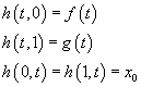
1. h(t, 0) = f(t)

2. h(t, 1) = g(t)

3. h(0, t) = h(1, t) = x₀

In other words, the function h can deform the function f into the function g, so that at time 0, the function h is the same as the function f, and at time 1, the function h is the same as the function g. So you can imagine the loop f deforming into the loop g over time, and the functions f and g are equivalent if this is possible. Such a function h is called a homotopy from f to g, and the corresponding equivalence classes are called homotopy classes.

The product f * g of two loops f and g is defined by setting

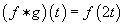
(f * g) (t) = f(2t)

if t is in [0, ½] and

(f * g) (t) = g(2t – 1)

if t is in [ ½, 1]

The loop f * g thus first follows the loop f with twice the speed, and then follows g with twice the speed. The product of two homotopy classes of loops [f] and [g] is then defined as [f * g] and it can be shown that this product does not depend on the choice of representatives. With this product, the set of all homotopy classes of loops with base point x₀ forms the fundamental group of X at the point x₀, and is written π₁(X, x₀). The identity is the constant map at the base point, and the inverse of loop f is the loop g defined by g(t) = f(1 – t), so g follows f backwards. Although the fundamental group in general depends on the base point, this choice makes no difference if X is path-connected, so you can write π₁(X) instead of π₁(X, x₀).

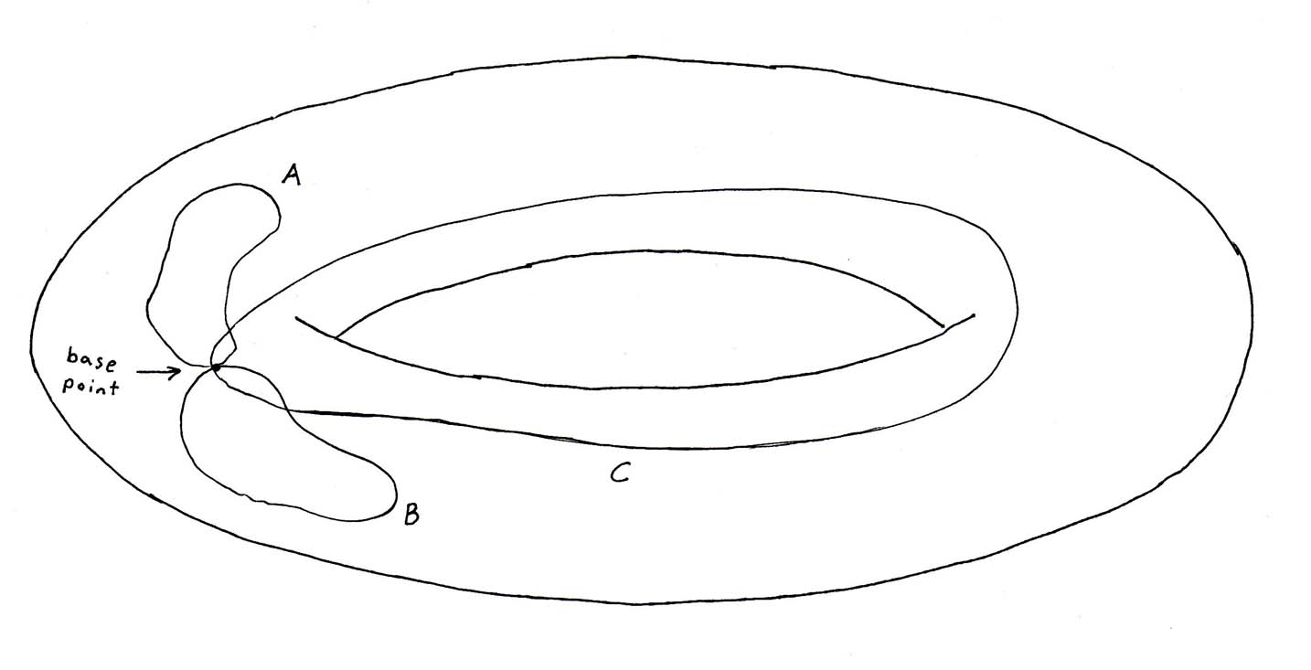
Here you have a torus with three possible loops drawn from a base point. Loops A and B can be deformed into each other, and could also be contracted to the base point. Loop C goes around the hole of the torus, and so could not be deformed into A or B, and can not be contracted to the base point. Therefore A and B are equivalent to the identity, while C is distinct. Notice that if we had used a sphere instead of a torus, then all loops could be deformed into each other, and all loops could be contracted to the base point.

There are some manifolds, such as a sphere or a plane, or any Sⁿ or Rⁿ, with n > 1, where any closed loop that could be drawn on the surface or in the space could always be contracted to a single point. In such a manifold, all loops, which are members of the group, can be contracted to the base point, and are thus equivalent to the identity, which is no movement at all. In other words, the group only has one member, which is the identity. This is the identity group which is the simplest possible group. A manifold on which any closed loop can be contracted to the base point is called simply-connected.

Then there are other manifolds where there is something the path can be taken around that prevents the loop from being shrunk to a single point. It could be a torus where the loop could wrap around the doughnut hole an integer number of times. A loop that wraps around the doughnut hole twice is distinct from a loop that wraps around it once. You would have the same thing with an infinite cylinder where the loop is perpendicular to the axis, or a punctured plane which is a plane with one point removed, or simply a circle, S¹, where the path could go an integer number of times around the circle. Each homotopy class consists of all loops which wind around the circle a given number of times, which can be positive or negative depending on the direction of the winding. The product of a loop that winds m times and another that winds n times is a loop that winds m + n times. Therefore the fundamental group of a circle is isomorphic to (Z, +), the additive group of the integers. If you have a circle, S¹, you could draw a path around the circle an integer number of times, so the fundamental group is the group of integers, represented by Z. In other words, π₁(S¹) = Z.

If you had a connected sum of two tori, which has genus 2, a loop could encircle one hole, or the other, or both of them, or do a figure eight between them, or any of the above any integer number of times. The greater the genus of the manifold, or the more boundaries or handles it has, the more complicated the resulting fundamental group.

The loop that forms the path that begins and ends at the base point, itself is topologically a circle, S¹. You can generalize this process from using S¹ to using Sⁿ, which is a sphere of any dimension. The resulting group is called the n-th homotopy group. When the path is a circle, S¹, the resulting group is the fundamental group, which is another name for the first homotopy group. You can use a sphere, S², instead of a circle, S¹, although in that case you can’t visualize it as a path traced by a point, and the resulting group is the second homotopy group. If you use an n-dimensional sphere, Sⁿ, it produces the n-th homotopy group π_n(X). In the sphere, Sⁿ, you choose a base point a. For a space X, with base point b, we define π_n(X) to be the homotopy classes of maps f : Sⁿ → X that map the base point a to the base point b. The equivalence classes are given by homotopies that are constant on the base point of the sphere. For n ≥ 1, the homotopy classes form a group. The first homotopy group, which is the fundamental group, is not abelian, but the higher homotopy groups, π_n(X) with n > 1, are abelian. This is because in two or more dimensions, two homotopies can be rotated around each other.

The group operations are not as simple as those for the fundamental group. Consider two maps a : Sⁿ → X and b : Sⁿ → X which pass through ρ ∈ X. The product a * b : Sⁿ → X is given by mapping the equator to the base point ρ. The northern hemisphere is mapped to the sphere by collapsing the equator to a point, and then it is mapped to X by a. The southern hemisphere is similarly mapped to X by b. The choice of direction of a loop in the fundamental group corresponds to a manifold orientation of Sⁿ in a homotopy group. Therefore the inverse of a map is given by switching orientation of the sphere. By describing the sphere in n + 1 coordinates, switching the first and second coordinates, changes the orientation of the sphere. Switching orientation reverses the roles of inside and outside. The homotopy groups do not depend on the choice of base point. Higher homotopy groups are abelian. The base point is fixed, and because n > 1, the map can be rotated. With n = 1, meaning the fundamental group, it’s impossible to rotate the map while keeping the base point fixed.

If you have a closed manifold where any loop can be contracted to a point, that means there are no boundaries or handles, which means it’s topologically a sphere. This is called the Poincare conjecture. This fact seems self-evidentially true but apparently it’s so difficult to prove that it was one of the Clay Institute’s Millennium Prizes. This was finally proven in 2006 by Grigory Perelman although he refused to accept any prize money because he doesn’t care about money, and instead cares only about advancing mathematics. Actually, it’s the 3D case that’s particularly difficult. It’s easy to prove in any other dimension.

A space with π(X) = 0 for all i ≤ n, is called n-connected. If X is n-1-connected, n > 1, then the Hurewicz homomorphism π(X) → H_n from the nth-homotopy group to the nth-homology group is an isomorphism.

When f : X → Y is a continuous map, then f_* : π_n(X) → π_n(Y) is defined by taking the images under f of the spheres in X. The push forward is natural.

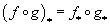
(f o g)_* = f_* o g

whenever the composition of two maps is defined. Given a fibration

F → E → B

Where B is pathwise-connected, there is a long exact sequence of homotopy groups

…→ π_n(F) → π_n(E) → π_n → π_{n – 1}(F) → …→ π₀(E) → π₀(B) = 0

Here the maps involving π₀ are not group homomorphisms because the π₀ are not groups but they are exact in the sense that the image equals the kernel. For example, let B equal S² and E equal S³. Let ρ be the Hopf fibration which has fiber S¹. From the long exact sequence

…→ π_n(S¹) → π_n(S³) → π_n(S²) → π_{n – 1}(S¹) →…

and the fact that π_n(S¹) = 0 for n ≥ 2, you have π_n(S³) = π_n(S²) for n ≥ 3. For instance, π₃(S²) = π₃(S³) = Z.

You also have relative homotopy groups π_n(X, A) for a pair (X, A). The elements of such a group are relative homotopy classes of maps Sⁿ → X. Two maps f and g are called homotopic to A if they are homotopic by a homotopy F : Sⁿ x [0, 1] &rarr X such that for each a in A, the map F(a, t) is constant. Normal homotopy groups are then a special case where A is the base point.

If M and N are topological spaces, then for their direct product you have

π_n(M x N) = π_n(M) x π_n(N)

If M is a simply-connected topological space, π₀(M) = π₁(M) = 0, and the group H acts on M, then you can form the topological space M/H identifying points of M which can be related by some elements H, where x = hx. You have

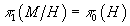
π₁1(M/H) = π₀(H)

In particular, if H is a discrete group π₀(H) and

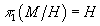
π₁(M/H) = H

For higher homotopy groups you have

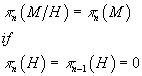
π_n(M/H) = π_n(M)

if π_n(H) = π(H) = π_{n – 1}(H) = 0

For a circle

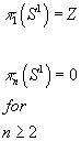
π₁(S¹) = Z

π_n(S¹) = 0

For higher dimensional spheres

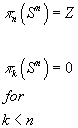
π_n(Sⁿ) = Z

π_k(Sⁿ) = 0 for k < n

Here are the homotopy groups for Sⁿ.

Sn	π1	π2	π3	π4	π5	π6	π7	π8	π9	π10
S1	Z	0	0	0	0	0	0	0	0	0
S2	0	Z	Z	Z2	Z2	Z12	Z2	Z2	Z3	Z15
S3	0	0	Z	Z2	Z2	Z12	Z2	Z2	Z3	Z15
S4	0	0	0	Z	Z2	Z2	Z x Z12	Z2 x Z2	Z2 x Z2	Z24 x Z3
S5	0	0	0	0	Z	Z2	Z2	Z24	Z2	Z2
S6	0	0	0	0	0	Z	Z2	Z2	Z24	0
S7	0	0	0	0	0	0	Z	Z2	Z2	Z24
S8	0	0	0	0	0	0	0	Z	Z2	Z2

For a torus

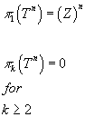
π₁(Tⁿ) = (Z)ⁿ

π_k(Tⁿ) = 0 for k ≥ 2

For real projective space

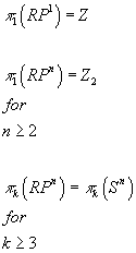
π₁(RP¹) = Z

π₁(RPⁿ) = Z₂ for n ≥ 2

π_k(RPⁿ) = π_k(Sⁿ) for k ≥ 2

For complex projective space

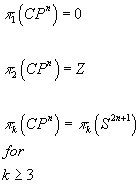
π₁(CPⁿ) = 0

π₂(CPⁿ) = Z

π_k(CPⁿ) = π_k(S^{2n + 1}) for k ≥ 3

I might mention in passing, the integers are symbolized by the letter Z because it stands for the German word “zahl” which means “to count”. This is, however, different from Zⁿ which is a symbol for an interval, which in that case stands for “Zyklus” which is the German word for “cycle”. In group theory, I use “I” to mean the identity, but some people use “e” and the reason is because it stands for “Einheit” which is the German word for “identity”. Later, I’ll discuss K-theory, where K stands for “Klassen” which is the German word for “class”.

The following capital English letters have π₁(X) = 0 since they don’t contain any closed loops.

C E F G H I J K L M N S T U V W X Y Z

The following capital English letters have π₁(X) = Z since they have one closed loop.

A D O P Q R

The following capital English letter has π₁(X) = Z x Z since it has two closed loops.

B

For the purpose of doing calculations in algebraic topology, a topological space is often approximated by a simplicial complex which is a lattice made up of points, line segments, triangles, tetrahedra, and their higher dimensional counterparts. A tetrahedron of arbitrary dimension is called a simplex, so triangles, tetrahedra, hypertetrahedra, etc, are types of simplices, and a lattice composed of these is a simplicial complex. For instance, a sphere could be approximated by an icosahedron which is then a simplicial complex in that it is composed of triangles. If the maximal dimension of the constituting simplices is k, then the complex is called a k-complex. An icosahedron would be a 2-complex. A simplicial complex is a combinatorial object telling you how to construct a topological space out of a number of simplices. A simplex by itself of dimension k is represented by labels called 0-simplices (its set of vertices), 1-simplices (line segments), 2-simplices (triangles), 3-simplices (tetrahedra), etc, all the way up to the single k-complex.

A simplicial complex is inadequate for some purposes, and so you can use a more general space called a CW-complex, which stands for closure finite weak complex. It involves gluing a closed n-dimensional ball Dⁿ to the (n – 1)-skeleton X_{n – 1}, which is the union all lower dimensional cells. A 0-cell is just a point. If you have only 0-cells building up a Hausdorff space, it must be a discrete space. It must be closure finite, meaning each closed cell should be covered by a finite union of open cells. We require that a subset C ⊂ X is closed when the intersection of C with the closed cells in X is always closed. This is called weak topology.

Given X₀ a discrete space, and inductively constructed subspaces X_i obtained from X_{i – 1} by attaching some collection of i-cells, the resulting colimit space X is called a CW-complex provided it is given the weak topology, and the closure finite condition is satisfied by its closed cells.

The idea of a homotopy category is to start with a topological space category, which is one in which the objects are topological spaces, and morphisms are continuous mappings, and to replace the sets Hom(X, Y) of morphisms by sets of equivalence classes HOT(X, Y) that are defined by the homotopy relation. So the objects remain the same but the morphisms have been gathered into collections.

The homotopy category of CW-complexes is the best, if not the only, candidate for the homotopy category. For technical reasons, a homotopy category must keep track of base points in each space. For example, the fundamental group of a connected space is dependent on the base point chosen. A topological space with a distinguished base point is called a pointed space.

In order to really do algebraic topology, you have to advance from homotopy groups to homology groups. Homology is a way to associate a sequence of abelian groups to a topological space. For a topological space, the homology groups are generally much easier to compute than the homotopy groups, so you will have an easier time working with homology when trying to classify spaces. Whereas each higher homotopy group has to be calculated independently, each homology group is defined in terms of the previous one.

You define a sequence of abelian groups A₀, A₁, A₂,… connected by homomorphisms

d_n : A_n → A_{n – 1}

such that the composition of any two consecutive maps is zero

d_n o d_{n + 1} = 0

for all n. This sequence is called a chain complex. This means that the image of the (n + 1)-th map is contained in the kernel of the n-th map, and we can define the n-th homology group X to be the factor group

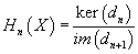
H_n(X) = ker(d_n)/im(d_{n + 1})

A chain complex is called exact if the image of the (n + 1)-th map is always equal to the kernel of the n-th map. The homology groups of X therefore measure how far the chain complex associated to X is from being exact.

Let’s say you have a simplicial complex X. Here A_n is the free abelian group whose generators are n-dimensional oriented simplices of X. The mappings are called the boundary mappings and send the simplices with vertices

(a[0], a[1], a[2],…a[n])

to the sum

[summation of i from 0 to n ](-1)ⁱ (a[0], …., a[i – 1], a[i + 1],…a[n])

If you take the modules to be over a field, then the dimension of the n-th homology of X turns out to be the number of holes in X at dimension n.

You can define a simplicial homology for any topological space X by defining a chain complex for X by taking A_n to be the free abelian group whose generators are all continuous maps from n-dimensional simplices into X. The homomorphisms d_n arise from the boundary maps of the simplices.

A homology group is an abelian group that partially counts the holes in a topological space. Singular homology groups form a measure of the hole structure of a space, but they are one particular measure, and they don’t always pick up everything.

The fundamental groups of a topological space X are related to its first singular homology group because a loop is also a singular 1-cycle. Mapping the homotopy class of each loop at its base point x₀ to the homology class of the loop gives a homomorphism from the fundamental group π₁(X, x₀) to the homology group H₁(X). If X is path-connected, then this homomorphism is surjective, and its kernel is the commutator subgroup of π₁(X, x₀), and H₁(X) is therefore isomorphic to the abelianization of π₁(X, x₀).

The Betti numbers of a topological space X are an infinite sequence of numbers, b₀, b₁, b₂,…,which are invariants of a topological space. Each Betti number is either a natural number, 0, 1, 2,…, or infinity. For most reasonable spaces, such as compact manifolds, finite simplicial complexes, or CW complexes, the sequence of Betti numbers, which consists of natural numbers, is zero from some point onwards, meaning all the Betti numbers after some point in the sequence are zero. The term “Betti numbers” was invented by Henri Poincare (1854 – 1912), and was named after Enrico Betti.

The k-th Betti number

b_k(X)

of the space X is defined as the rank of the abelian group

H_k(X)

The k-th homology group of X.

You can also define it as a vector space dimension of

H_k(X, Q)

Since the homology group in this case is a vector space over Q. The universal coefficient theorem shows that these definitions are the same.

More generally, given a field F, you can define

b_k(X, F)

the k-th Betti number with coefficient in F, as the vector space dimension of

H_k(X, F)

The Betti numbers b_k(X) do not take into account any torsion in the homology groups, but they are still very useful. Basically, they allow you to count the number of holes of different dimensions. For a circle, the first Betti number is 1. For a general pretzel, the first Betti number is twice the number of holes. In the case of a finite simplicial complex, the homology groups H_k(X, Z) are finitely-generated, and so have a finite rank. The rank of the group is zero when k exceeds the dimension of a simplex of X.

For a finite CW-complex K, you have

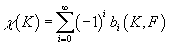
χ(K) = [summation over i from 0 to infinity] (-1)ⁱb_i(K, F)

where χ(K) is the Euler characteristic of K and any field F.

For any two spaces X and Y, you have

P_{X x Y} = P_XP_Y

Where P_X is the Poincare polynomial of X, which is the generating function of the Betti numbers of X.

P_X = b₀(X) + b₁(X)z + b₂(X)z² + …

If X is an n-dimensional manifold, there is a symmetry interchanging k and n – k, for any k.

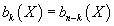
b_k(X) = b_{n – k}(X)

The dependence on the field F is only through its characteristic. If the homology groups are torsion-free, the Betti numbers are independent of F. The connection of p-torsion and the Betti number for a characteristic p, where p is a prime number, is given in detail by the universal coefficient theorem.

The Betti number sequence for a point, R⁰, is

1, 0, 0, 0,…

The Betti number sequence for a circle, S¹, is

1, 1, 0, 0, 0,…

The Betti number sequence for a two-torus, T², is

1, 2, 1, 0, 0, 0….

The Betti number sequence for a three-torus, T³, is

1, 3, 3, 1, 0, 0, 0,…

The Betti number sequence for a four-torus, T⁴ is

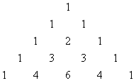
1, 4, 6, 4, 1, 0, 0, 0,…

Notice this reproduces Pascal’s Triangle, invented by Blaise Pascal (1632 – 1662)

               1
            1	  1
        1     2     1
     1     3      3     1
1      4     6       4      1

where each number is the sum of the two numbers directly above it, with zeroes off the diagonal. The numbers in line n are the coefficients you get if you expand (x + y)ⁿ. Also, if you draw Pascal’s Triangle, and color in the odd entries, you get a fractal called Sierpinski’s Gasket.

When Pascal wrote about Pascal’s Triangle in 1654, he was merely rediscovering it. The basic idea of Pascal’s triangle goes back to Mersenne in 1636, and Tartaglia in 1556, and the Hindu mathematician Bhaskara in 1150, and the Jain mathematician Mahavira in 850 A. D.

For any Rⁿ, such as a point, line, plane, 3D space, 4D space, etc, or any subunit thereof, such as an interval, disk, ball, etc, the first Betti number is 1, and the rest are zero.

It’s possible for spaces that are infinite-dimensional to have an infinite series of non-zero Betti numbers. An example is the infinite-dimensional complex projective plane, which has a sequence of 1, 0, 1, 0,…. which is periodic with period length 2. Here are examples of the Betti numbers of manifolds.

1. b_n(S¹) = 1, 1, 0, 0, 0,…

2. b_n(T²) = 1, 2, 1, 0, 0, 0,…

3. b_n(T³) = 1, 3, 3, 1, 0, 0, 0,…

4. b_n(Rⁿ) = 1, 0, 0, 0, 0,…

5. b_n(CP^∞) = 1, 0, 1, 0, 1, 0,…

Also, Betti numbers predict the dimensions of vector spaces of closed differential forms. The connection with the definition given above is from three different results, which are de Rham’s theorem, Poincare’s duality, and the universal coefficient theorem. You could also say that Betti numbers give the dimensions of spaces of harmonic functions, which requires results from Hodge theory, and the Hodge Laplacian.

The Euler characteristic of any topological space is defined as an alternating sum of its Betti numbers.

χ = b₀ – b₁ + b₂ – b₃ +…

Here are the Euler characteristics for the manifolds listed above.

1. χ(S¹) = 1 – 1 + 0 – 0 +… = 0

2. χ(T²) = 1 – 2 + 1 – 0 + 0 – … = 0

3. χ(T³) = 1 – 3 + 3 – 1 + 0 -… = 0

4. χ(Rⁿ) = 1 – 0 + 0 – 0 + 0 -… = 1

5. χ(CP^∞) = 1 – 0 + 1 – 0 + 1 -…= ∞

In my paper “Beyond the Standard Model”, I give the Betti numbers and Euler characteristic of a Calabi-Yau manifold.

If the topology is approximated by CW-complex, the above definition reduces to the alternating sum

χ = k₀ – k₁ + k₂ – k₃ +…

where k is the number of cells of dimension n in the complex.

A polytope is a type of CW-complex, where the manifold it approximates is Sⁿ. A polyhedron is a CW-complex where k₀ is the number of vertices, k₁ is the number of edges, and k₂ is the number of faces. The above formula then reduces to

χ = V – E + F

where V is the number of vertices, E is the number of edges, and F is the number of faces. Polyhedra are homeomorphic to a sphere, S², which has an Euler characteristic of 2, so therefore

V – E + F = 2

which is the original Euler’s formula. This famous formula was discovered by Leonard Euler (1707 – 1783), one of the greatest mathematicians. Originally from Switzerland, he went to St. Petersburg at the request of Catherine the Great, who also hosted the mathematician Dennis Diderot, and corresponded with Voltaire. Euler then went to Prussia, and served as mathematician for Frederick the Great. After he lost sight in one of his eyes, Frederick called him his “mathematical cyclops”. Euler returned to St. Petersburg where he went completely blind. Incidentally, Voltaire also had an adulterous affair with Emily du Chatalet who, as one of the few female scientists before the late 19th Century, helped determine that the energy of a body is proportional to its velocity squared.

The Euler characteristic of a compact 2D manifold can be calculated from

χ = 2 – 2g – b – k

where g is the genus or number of handles, b is the number of boundaries, and k takes into account the possibility of the manifold being non-orientable. The genus g is technically defined as the number of tori in a connected sum of the surface. Similarly, k is the number of projective planes in a connective sum of the surface.

Here are some examples.

1. For sphere, S², you have

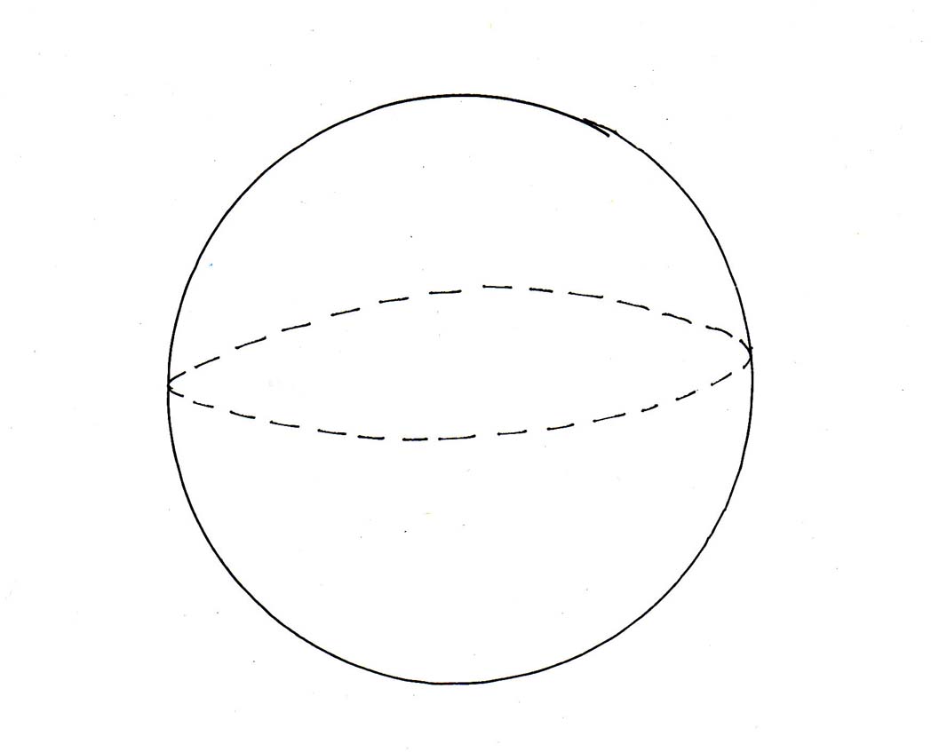
χ = 2 – 2g – b – k

χ = 2 – 2(0) – (0) – (0) = 2

2. For a torus, T², you have

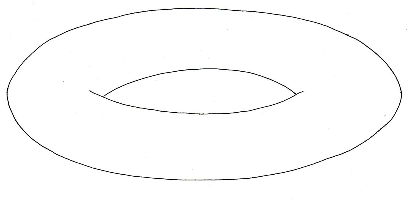
χ = 2 – 2g – b – k

χ = 2 -2(1) – (0) – (0) = 2 – 2 = 0

3. For a finite cylinder, S¹ x I, you have

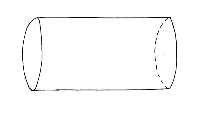
χ = 2 – 2g – b – k

χ = 2 -2(0) – (2) – (0) = 2 – 2 = 0

4. For a Klein bottle, KB, you have

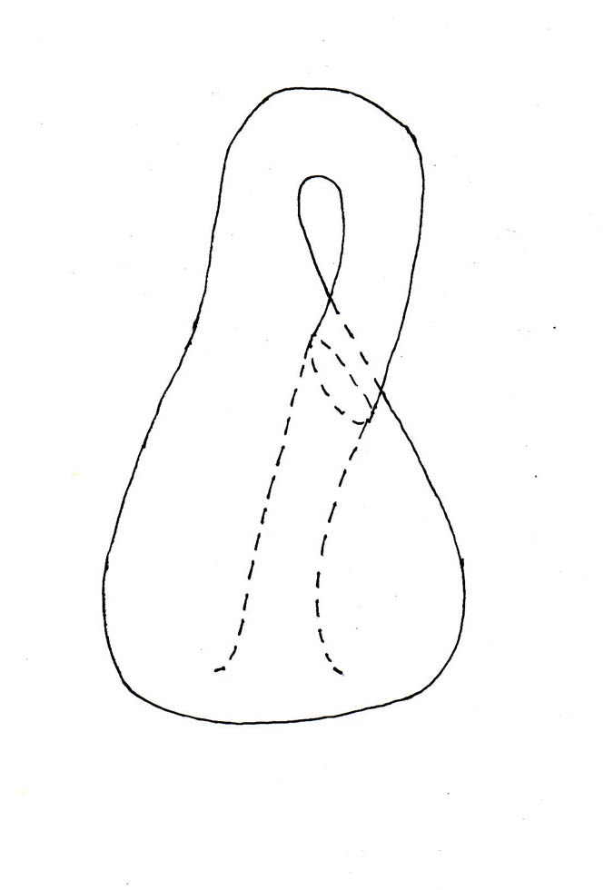
χ = 2 – 2g – b – k

χ = 2 – 2(0) – (0) – (2) = 2 – 2 = 0

5. For a Möbius strip, MS, you have

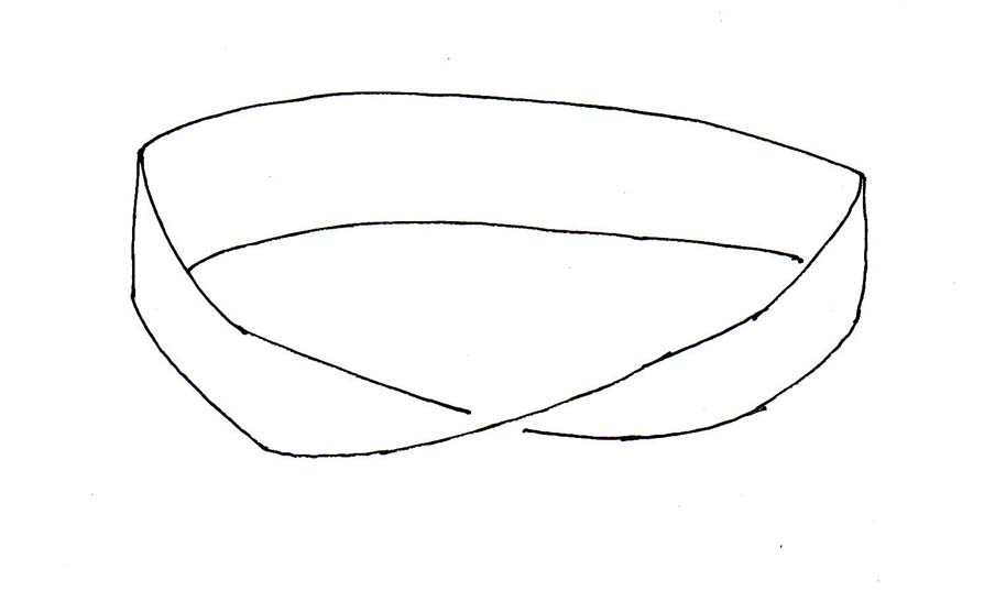
χ = 2 – 2g – b – k

χ = 2 – 2(0) – (1) – (1) = 2 – 1 – 1 = 0

6. For a Roman surface, you have

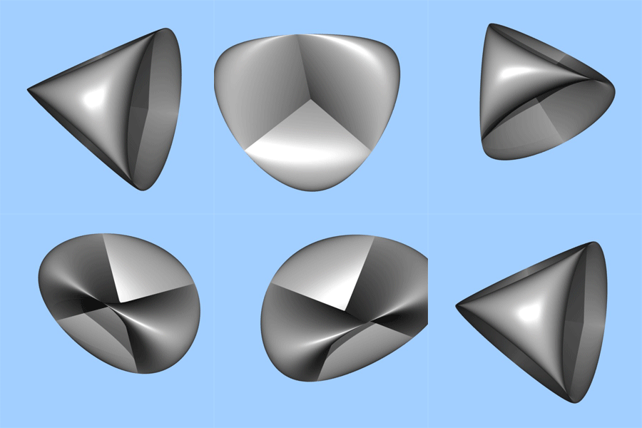
χ = 2 – 2g – b – k

χ = 2 – 2(0) – (0) – (1) = 2 – 1 = 1

7. For a double torus, T² # T², you have

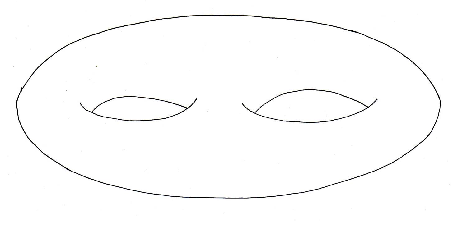
χ = 2 – 2g – b – k

χ = 2 – 2(2) – (0) – (0) = 2 – 4 = -2

8. For a “pair of pants”, you have

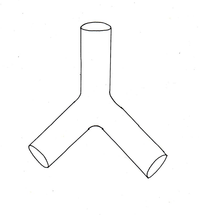
χ = 2 – 2g – b – k

χ = 2 – 2(0) – (3) – (0) = 2 – 3 = -1

The Euler characteristic of the disjoint union of two unconnected manifolds is simply the sum of their Euler characteristics, so the Euler characteristic of two spheres is 2 + 2 = 4.

Let’s go back to this definition.

χ = b₀ – b₁ + b₂ – b₃ +…

Any contractible space Rⁿ has trivial homology, meaning the 0th Betti number is 1, and all others 0. Therefore, its Euler characteristic is 1. This includes Rⁿ of any dimension, as well as finite subgroups thereof, such as interval, disk, ball, etc. Any polytope of any dimension, such as any point, line segment, polygon, polyhedron, polychoron (4D polytope), etc, as well as any finite lattice thereof, such as a checkerboard, Rubik’s cube, finite honeycomb, kagome lattice, etc, will obey

V – E + F – C + HC – … = 1

where V is the number of vertices, E is the number of edges, F is the number of faces, C is the number of cells, HC is the number of hypercells, etc, as long as you count the interior, so a line segment would be considered to have one edge, a polygon would be considered to have one face, a polyhedron would be considered to have one cell, etc. In that case, the polytope or finite lattice would be topologically equivalent to a finite subunit of Rⁿ, such as a disk or ball, and would therefore have an Euler characteristic of 1. If you take the absolute value of series, then it will also work for any Rⁿ, such as a point, line, plane, 3D space, 4D space, etc, as well unbounded polytopes, such as a wall, chimney, etc.

In homology, if (d_n : A_n → A_{n – 1}) is a chain complex such that all but a finitely many A_n are zero, and the others are finitely generated abelian groups, or finite dimensional vector spaces, then you can define the Euler characteristic as

χ = [summation] (-1)ⁿ rank (A_n)

using the rank in the case of the abelian groups, or the Hamel dimension in the case of vector spaces. It turns out that the Euler characteristic can also be computed at the level of homology.

χ = [summation] (-1)ⁿ rank (H_n)

This provides two ways to compute χ for the object X which gave rise to the chain complex. Every short exact sequence

0 → A → B → C → 0

of chain complexes gives rise to a long exact sequence of homology groups

…→ H_n(A) → H_n(B) → H_n(C) → H_{n – 1}(A) → H_{n – 1}(B) → H_{n – 1}(C) → H_{n – 2}(A) → …

All maps in this long exact sequence are induced by the maps between the chain complexes, except for the maps H_n(C) → H_{n – 1} (A). These are called connecting homomorphisms and are provided by the snake lemma.

If X is a topological space, and ABC ⊂ X are such that X = int (A) ∪ int (B) and C = A ∩ B, then there is an exact sequence of homology groups

…→ H_n(C) → H_n(A) + H_n(B) → H_n(X) → H_{n – 1}(C) →…

where i_* is induced by the inclusions i : B → X and j_* by j : A → X, and ∂_* is the following map. If X is in H_n(X), then it can be written as a sum of a chain in A, and one in B, x = a + b, ∂x = -∂b, since ∂x = 0. Thus, ∂a is a chain in C, and so is a class in H_{n – 1}(C). This is ∂_*X. You can easily check by standard diagram chasing that this map is well defined on the level of homology. This sequence is called the Mayer-Vietoris sequence.

The Mayer-Vietoris sequence, named after Walter Mayer and Leopold Vietoris, is an exact sequence that you can use to compute homology groups. It’s somewhat analogous to the Siefert-van Kampen theorem for homotopy groups. Homology groups can be computed directly using the tools of linear algebra in simplicial homology. However, such calculations can be very cumbersome, and it’s great to have a way to compute homology groups from other ones that you already have. The Mayer-Vietoris sequence is the easiest way to do this.

For a topological space X with two subsets U and V, whose union is X, we call (X, U, V) a triad. It’s sometimes possible to form triads out of non-open subsets but it doesn’t always work. The Mayer-Vietoris sequence of the triad (X, U, V) is a long exact sequence which relates the singular homology groups of the space X to those of U, V, and their intersection A.

…→ H_{n + 1}(X) →(∂) H_n(A) →(φ) H_n(U) + H_n(V) →(ψ) H_n(X) →(∂) H_{n – 1}(A) → …

where H_n(X) is the n-dimensional homology group of the space X. The maps between each homology group of the same dimension n are induced by the inclusions of A into U, and U and V into X. More precisely, the map φ into the direct sum is a product map, and the map ψ out of the direct sum is a difference. The map ∂ that lowers the dimension is a boundary map that comes from the snake lemma.

One application of the Mayer-Vietoris sequence is to prove that the n-th reduced homology group of the sphere S^k is trivial unless n = k, in which case H_k(*S^k) is isomorphic to the group of integers Z. Here you have a complete classification of homology groups for spheres, in contrast to what is known for the homotopy groups of spheres. There is a similar result for n < k, but not much is known for n > k.

The morphisms in homology are called functors. A functor is a special type of mapping between categories. A covariant functor, which is what people mean when they just say “functor”, is defined as follows.

Let C and D be categories. A functor F from C to D is a mapping that

1. Associates to each object X in C an object F(x) in D.

2. Associates to each morphism f : X → Y in C, a morphism F(f) : F(X) → F(Y) in D.

such that the following two properties hold

1. F(id_X) = id_F(X) for every object X in C.

2. F(g o f) = F(g) o F(f) for all morphisms f : X → Y and g : Y → Z.

In other words, functors preserve identity morphisms and composition of morphisms.

So you see that a functor just says that for every object and morphism in one category, you have a corresponding object and morphism in the other category. A contravariant functor, also called a cofunctor, is the same except the corresponding morphism in the other category goes in the opposite direction, from Y to X instead of X to Y.

Let C and D be categories. A contravariant functor F from C to D is a mapping that

1. Associates to each object X in C an object F(x) in D.

2. Associates to each morphism f : X → Y in C, a morphism F(f) : F(Y) → F(X) in D.

such that the following two properties hold

1. F(id_X) = id_F(X) for every object X in C.

2. F(g o f) = F(g) o F(f) for all morphisms f : X → Y and g : Y → Z.

In other words, cofunctors preserve identity morphisms and composition of morphisms.

You can also define a contravariant functor as a covariant functor on a dual category C^op. Some people prefer to write all expressions covariantly, so instead of saying F : C → D is a contravariant functor, they would say F : C^op → D or F : C → D^op and call it a covariant functor.

The different types of categories that functors act on could be sets, represented by “Set”, categories, represented by “Cat”, groups, represented by “Grp”, abelian groups, or “Ab”, rings or “Rng”, group homomorphisms or “Hom”, topology or “Top”, algebra or “Alg”, etc. For instance, λCalc → Cart is a functor from a typed λ-calculus to a cartesian closed category. Top → Phas is a functor from a target space to a phase space. 2Cob → Vect_K is a functor from the category of 2-dimensional cobordisms to the category of vector spaces over K.

Forgetful functors are functors that go from an object with more structure to an object with less structure, so it “forgets” some structure. One example is the functor U : Grp → Set, which maps from a group to a set. In other words, it “forgets” the binary operation, leaving only the members of the group, which without a binary operation, now form a set. Another example is the functor Rng → Ab, which maps from a ring to its underlying abelian group. Going in the opposite direction from forgetful functors are free functors. The free functor Set → Grp sends every set X to the free group generated by X. Functions get mapped to group homomorphisms between free groups. The extra structure that is added during the morphism is unspecified by the original and is thus “free” to take any value.

To every pair A, B of abelian groups, you can assign the abelian group Hom(A, B) consisting of all group homomorphisms from A to B. This is a functor which is contravariant in the first, and covariant in the second, argument. It is a functor Ab^op x Ab → Ab where Ab denotes the category of abelian groups with group homomorphisms. If f : A₁ → A₂ and g : B₁ → B₂ are morphisms in Ab, then the group homomorphism Hom(f, g) : Hom (A₂, B₁) → Hom(A₁, B₂) is given by φ | → g o φ o f.

You can generalize this is any category C. To every pair X, Y of objects in C, you can assign the set Hom(X, Y) of morphisms from X to Y. This defines a functor to Set which is contravariant in the first argument, and covariant in the second argument. This is a functor C^op x C → Set. If f : X₁ → X₂ and g : Y₁ → Y₂ are morphisms in C, then the group homomorphism Hom(f, g) : Hom(X₂, Y₁) → Hom(X₁, Y₂) is given by φ | g o φ o f.

If X is a topological space, then the open sets in X form a partially ordered set Open(X) under inclusion. Like every partially ordered set, Open(X) forms a small category by adding a single arrow U → V if and only if U is a subset of V. Contravariant functors on Open(X) are called presheaves on X. For instance, by assigning to every open set U the associative algebra of real-valued continuous functions on U, you get a presheaf of algebras on X.

On any category C, you can define the identity functor 1_C, which maps every object and morphism to itself. You can also define the constant functor, C → D which maps every object in C to a specific object X in D, and every morphism in C to the identity morphism on X. You can compose functors. If F is a functor from A to B, and G is a functor from B to C, then you can form the composite functor GF from A to C. Composition of functors is associative where defined. This shows that functors can be considered as morphisms in categories of categories.

Functors themselves can be considered as objects in a category called a functor category. Morphisms in this category are natural transformations between functors. You can then have functors acting between functor categories. The diagonal functor is defined as the functor from D to the functor category D^C which sends each object in D to the constant functor at that object.

Chain complexes form a category. A morphism from the chain complex d_n : A_n → A_{n – 1} to the chain complex e_n : B_n → B_{n – 1} is sequence of homomorphisms f_n : A_n → B_n such that f_{n – 1} * d_n = e_{n – 1} * f_n for all n. The n-th homology H_n can be viewed as a covariant functor from the chain complexes to the category of abelian groups.

If the chain complex depends on the object X is a covariant manner, meaning that any morphism X → Y induces a morphism from the chain complex of X to the chain complex of Y, then the H_n are covariant functors from the category it belongs to into the category of abelian groups.

In homology, the chain complexes depend in a covariant manner on X, and the homology groups form covariant functors. If instead, you assume that the chain complexes depend in a contravariant way on X, the homology groups form contravariant functors. The resulting subject is called cohomology. When you go from covariant functors to contravariant functors, you go from homology to cohomology. You refer to the chains as cochains, and the groups as cohomology groups. Cohomology can be viewed as a method of assigning algebraic invariants to a topological space that has a more refined structure than does homology. Cohomology arises from the algebraic dualization of the construction of homology. Homology and cohomology are duals of each other. You could also say that the cochains in cohomology should assign quantities to the chains in homology.

Homology began in the late 19th Century. They thought of a k-chain as a formal combination

[summation] a_id_i

where a_i are integers, and d_i are k-dimensional simplices on X. For instance, if X is a two-torus T², a one-dimensional cycle on T² is intuitive in terms of a linear combination of curves drawn on T², which closes up on itself, obeying the cycle condition, meaning having no boundary. If C and D are cycles each wrapping once around T² the same way, you can find an oriented surface on T² with boundary C-D. Topologists can prove that the homology classes of 1-cycles with integer coefficients form a free abelian group with two generators, one for each of the two different ways around a torus.

This is the 19th Century view based on the Riemann surface. This view was made more general by Henri Poincare who first stated the general Stoke’s theorem in 1899. It involves both an integrand, called a differential form, and a region of integration, called a p-chain, with two kinds of boundary operators, one of which is the exterior derivative, and the other a geometric boundary operator on chains that includes orientation, and can be used for homology theory. The two boundaries appear as adjoint operators with respect to integration.

Geometrical arguments with homology were only gradually replaced by rigorous techniques in the early 20th Century. Originally, they used combinatorial topology which assumes that the spaces that are treated are simplicial complexes while the most interesting spaces are manifolds so that artificial triangulations have to be introduced to apply the tools. Combinatorial topology allowed Brouwer to prove the simplicial approximation theorem, which is based on the idea that homology is a functor. Brouwer also proved the Jordan curve theorem, and the invariance of domain.

The transition from combinatorial topology to algebraic topology is attributed to Emmy Noether who said that homology classes are in quotient groups. Emmy Noether, in the period from 1920 onwards, was with her students elaborating the theory of modules for any ring. The ideas of homology and rings were combined to give the idea of homology with coefficients in a ring. The coefficients are the way in which chains are linear combinations of the basic geometric chains traced on the space. Originally, they had been assumed to be integers. Then they could be viewed as integers, real, or complex numbers, or possibly residue classes mod 2. However, with the recent developments by Emmy Noether, they could, for instance, be residue classes mod 3. Then the cycle would be a more complicated geometrical situation where the number of incoming edges at every vertex has to be multiple of 3. The universal coefficient theorem determines all other homology theories through the tensor product.

During the 1930s, you had the development of cohomology theories. Several research directions came together, and the de Rham cohomology that was implicit in Poincare’s work became the subject of definite theorems. Homology and cohomology are dual theories. The details required working out. Also, singular homology avoided the need for the apparatus of triangulations, although this required using infinitely generated modules.

From 1940 to 1960, the subject of algebraic topology advanced very rapidly. Homology theory was often used as a baseline theory, easy to compute, and in terms of which topologists sought to calculate other functors. The axiomatisation of homology theory by Eilenberg and Steenrod showed that what various homology theories had in common was some exact sequences, such as the Mayer-Vietoris theorem, and the dimension axiom, which calculated the homology of a point. Then the dimension axiom was relaxed to admit cohomology derived from topological K-theory and cobordism. This vastly extended cohomology to include extraordinary cohomology theories, that became standard in homotopy theory. These can be easily characterized for the category of CW complexes. For more general spaces, recourse to sheaf theory brought some extension of homology theories, such as the Borel-Moore theory for locally compact spaces.

Cohomology is a general term for a sequence of abelian groups defined from a cochain complex. Cohomology is defined as the abstract study of cochains, cocycles, and coboundaries. Cohomology can be viewed as a method of assigning algebraic invariants to a topological space that has a more refined algebraic structure than homology. Cohomology arises from the algebraic dualization of homology. Cochains should assign quantities to the chains in homology.

From its beginning in topology, this idea became a dominant method in the mathematics of the second half of the 20th Century. For many applications, cohomology, a contravariant theory, is more natural than homology. This has to do with functors and pullbacks in geometric situations. Given spaces X and Y, and some kind of functor F on Y, for any mapping f : X → Y, composition with f gives rise to a functor F o f on X. Cohomology groups also have natural products, makin calculation easier.

Although cohomology is fundamental to modern algebraic topology, its importance was not realized until 40 years after the development of homology. The concept of dual cell structure, which Henri Poincare used in his proof of the Poincare duality theorem, contained the origin of the idea of cohomology, but this was not realized until later.

There were various precursors to cohomology. In the 1930s, J. W. Alexander and Lefschetz founded the intersection theory of cycles on manifolds. On an n-dimensional manifold M, a p-cycle and a q-cycle with non-empty intersection, will, if in a general position, have an intersection of a (p + q – n)-cycle. Therefore, you can define a multiplication of homology classes.

H_p(M) x H_q(M) → H_{p + q – n}(M)

Here is a brief chronology of cohomology.

1. In 1893, Henri Poincare used what was later recognized to be a reference to cohomology to prove the Poincare duality theorem.

2. In 1930, Alexander defined the cochain based on a p-chain on a space X having relevance to small neighborhoods of the diagonal in X^{p + 1}.

3. In 1931, de Rham related homology and exterior differential forms, proving de Rham’s theorem. This result is now understood to be more naturally interpreted in terms of cohomology.

4. In 1934, Pontrjagin proved the Pontrjagin duality theorem, which is a result on topological groups. This, in special cases, provided an interpretation of Poincare’s duality and Alexander’s duality in terms of group characters.

5. In a 1935 conference in Moscow, Kolmogorov and Alexander both introduced cohomology, and tried to construct a cohomology product structure.

6. In 1936, Steenrod published a paper constructing Cech cohomology by dualizing Cech homology.

7. From 1936 to 1938, Hassler Whitney and Eduard Cech developed the cup product, making cohomology into a graded ring, and the cap product, and realized that Poincare duality can be stated in terms of the cap product. Their theory was still limited to cell complexes.

8. In 1944, Eilenberg overcame technical limitations, and gave the modern definition of singular homology and cohomology.

9. In 1945, Eilenberg and Steenrod stated the axioms defining a homology and cohomology theory.

10. In 1948, Spanier, building on work of Alexander and Kolmogorov, developed Alexander-Spanier cohomology.

11. In 1952, Eilenberg and Steenrod publish “Foundations of Algebraic Topology”, where they prove that the existing homology and cohomology theories satisfied their axioms.

12. In 1959, Jean-Pierre Serre used the analogy of vector bundles with projective modules to create algebraic K-theory.

A cohomology theory is a family of contravariant functors from the category of pairs of topological spaces and continuous functions, or some subcategory thereof, such as the category of CW complexes, to the category of abelian groups and group homomorphisms that satisfies the Eilenberg-Steenrod axioms.

The Eilenberg-Steenrod axioms apply to a sequence of functors H_n from the category of pairs of topological spaces to the category of abelian groups, together with a natural transformation

∂ : H_i(X, A) → H_{i – 1}(A)

called the boundary map. The Eileen-Steenrod axioms are

1. Homotopy – Homotopic maps induce the same maps in homology.

2. Excision – If (X, A) is a pair and U is contained in the interior of A, then the inclusion map

i : (X – U, A – U) → (X, A)

induces an isomorphism in homology.

3. Let P be the one-point space. Then H_n(P) = 0 for all n ≠ 0.

4. Addivity – If

X = V_α X_α

then

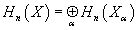
H_n(X) = [direct sum series over α] H_n(X_α)

5. Exactness – Each pair (X, A) induces a long exact sequence in homology via the inclusions i : A → X and j : X → (X, A)

…→ H_n(A) →(i) H_n(X) →(j) H_n(X, A) →(∂) H_{n – 1}(A) → …

If P is the one point space then H₀(P) is called the coefficient group. For instance, singular homology has integer coefficients.

Some facts about homology groups can be derived directly from the axioms, such as the fact that homotopically equivalent spaces have isomorphic homology groups. The homology of some relatively simple spaces, such as n-spheres, can be calculated directly from the axioms. From this, it can be easily shown that the (n – 1)-sphere is not a retract from the n-disk.

The main cohomology theories that satisfy the Eilenberg-Steenrod axioms are

1. simplicial cohomology

2. singular cohomology

3. de Rham cohomology

4. Čech cohomology

5. Sheaf cohomology

6. Alexander-Spanier cohomology

Let’s say you take the Eilenberg-Steenrod axioms that I just listed, and you relax axiom #3, meaning that you allow cohomology theories that do not obey the third axiom but do obey the others. The third axiom is

3. Let P be the one-point space. Then H_n(P) = 0 for all n ≠ 0.

Relaxing this condition gives rise to a new type of cohomology theory called extraordinary cohomology theory. This allows theories based on K-theory and cobordism theory, as well as other theories coming from stable homotopy theory.

Since the axioms that extraordinary cohomology theories obey are less restrictive than those that traditional cohomology theories obey, there are therefore a lot more of them. The main extraordinary cohomology theories include

1. Group cohomology

2. Galois cohomology

3. Lie algebra cohomology

4. Harrison cohomology

5. Γ cohomology

6. Schur cohomology

7. Andre-Quillen cohomology

8. Hochschild cohomology

9. Cyclic cohomology

10. Topological Andre-Quillen cohomology

11. Topological Hochschild cohomology

12. Topological Cyclic cohomology

13. Coherent cohomology

14. Local cohomology

15. Etale cohomology

16. Crystalline cohomology

17. Flat cohomology

18. Motive cohomology

19. Deligne cohomology

20. Perverse cohomology

21. Intersection cohomology

22. Non-abelian cohomology

23. Gel’fand-Fuks cohomology

24. Spencer cohomology

25. Bonar-Claven cohomology

26. K-theory

The most famous cohomology theory is de Rham cohomology, invented by Georges de Rham, which is a cohomology theory based on the existence of differential forms with prescribed properties. It is, in different ways, dual to both singular homology and Alexander-Spanier cohomology.

Let’s say you have a set of smooth differentiable differential k-forms on any smooth manifold M which form an abelian group, which is a real vector space called

Ω^k(M)

under addition. The exterior derivative d gives mappings

d : Ω^k(M) → Ω^{k + 1}(M)

There is a fundamental relationship

d² = 0

which follows from the symmetry of second derivatives. Therefore vector spaces of k-forms along with the exterior derivative are a cochain complex called the de Rham complex

C^∞(M) = Ω⁰(M) → Ω¹(M) → Ω²(M) → Ω³(M) →…

Forms that are exterior derivatives are called exact. Forms whose exterior derivatives are zero are called closed. The relationship d² = 0 then says that exact forms are closed.

Of course, closed forms don’t have to be exact. The idea of de Rham cohomology is to classify the different types of closed forms on a manifold. Two closed forms α and β in Ω^k(M) are called cohomologous if they differ by an exact form, in other words, if α – β is exact. This means that there is an equivalence relation on the space of closed forms in Ω^k(M). You then define the k-th de Rham cohomology group

H_dR^k(M)

To be the set of equivalence classes, which is the set of closed forms in Ω^k(M) modulo the exact forms.

For any manifold M with n connected components

H_dR⁰ = Rⁿ

Where the equal sign means that the two are homeomorphic. This follows from the fact that any C^∞ function on M with zero derivative is locally constant on each of the connected components.

You can find the general de Rham cohomologies of a manifold by using the above fact about zero cohomology and the Mayer-Vietoris sequence, and also the fact that de Rham cohomology is homotopy invariant.

Here are the de Rham cohomology groups of some topological spaces.

1. sphere, Sⁿ

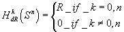
H_dR^k(Sⁿ) = R if k = 0, n, and = 0 if k ≠ 0, n

2. torus, Tⁿ

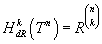
H_dR^k(Tⁿ) = R^{(n, k)}

3. punctured plane, R² – {(0, 0)}

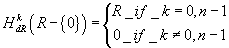
H_dR^k( R² – {(0, 0)}) = R if k = 0, n – 1, and = 0 if k ≠ 0, n – 1

4. Möbius strip, MS

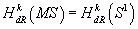
H_dR^k = H_dR^k(S¹)

De Rham’s theorem, proved by Georges de Rham in 1931, states that for a compact oriented smooth manifold M, the groups H_dR^k(M) are isomorphic as real vector spaces with singular cohomology groups.

H_dR^k = (M ; R)

The wedge product endows the direct sum with a ring structure. A further result of the theorem is that two cohomology rings are isomorphic, as graded rings, where the analogous product on singular cohomology is the cup product. The general Stokes theorem is an expression of duality between de Rham cohomology and the homology of chains.

The first extraordinary cohomology theory was K-theory. It includes both topological K-theory and algebraic K-theory. It leads to the construction of K-functors which contain useful information, which is, however, often difficult to compute. K-theory was originally discovered/invented by Alexander Grothendieck so he could formulate his Grothendieck-Riemann-Rock theorem. K-theory stands for Klassen-theory, where “Klassen” is the German word for “class”. Grothendieck needed to convert the commutative monoid of sheaves with an operation of direct sum into a group. Instead of attempting to work with sheaves directly, he took formal sums of certain classes of sheaves and formally added inverses. This is an explicit way of obtaining a left adjoint of a certain functor. This construction is called the Grothendieck group. It was taken up by Michael Atiyah and Friedrich Hirzebruch to define K(X) for a topological space X by means of the analogous sum construction for vector bundles. This was the basis of the first of the extraordinary cohomology theories of algebraic topology. It played a big role in the second proof of the Index Theorem in 1962. This approach also led to a noncommutative K-theory for C*-algebra.

In 1959, Jean-Pierre Serre used the analogy of vector bundles with projective modules to create algebraic K-theory. He formulated Serre’s conjecture, that projective modules over the ring of polynomials over a free field are modules. This resisted proof for 20 years. There then followed a period in which there were various partial definitions of higher K-functors until a comprehensive definition was given by Daniel Quillen using homotopy theory. The corresponding constructions involving an auxiliary quadratic form are called L-theory. It is a major tool in surgery theory.

Topological K-theory is the true K-theory in the sense that it came first. Topological K-theory has to do with vector bundles over topological spaces. Elements of K-theory are stable equivalence classes of vector bundles over a topological space. You can put a ring structure on the collection of stably equivalent bundles by defining addition through the Whitney sum, and multiplication through the tensor product of vector bundles. This defines the reduced real topological theory of a space. Of course, you could also use complex vector bundles instead of real vector bundles. Topological K-theory is significant because it forms a generalized cohomology theory, and it leads to a solution of the vector fields on a sphere problem, as well as to an understanding of the J-homeomorphism of homotopy theory.

In 1962, Swan noticed that there is a correspondence between the category of suitable topological spaces, such as Hausdorff spaces, and C*-algebras. The idea is to associate to every space the C*-algebra of continuous maps from that space to the reals. A vector bundle over a space has sections, and these sections can be multiplied by continuous functions to the reals. According the Swan’s correspondence, vector bundles correspond to modules over the C*-algebra of continuous functions, the modules being the modules of sections of the vector bundle. The study of modules over C*-algebras is the starting point of algebraic K-theory. The Quillen-Lichtenbaum conjecture connects algebraic K-theory to Etale cohomology.

Alexander Grothendieck suddenly disappeared in 1991. Nobody knew if he was alive or dead. His whereabouts or ultimate fate were the source of endless speculation in the mathematical community. However, it turned out that he became a hermit, and is living in seclusion because he’s embarrassed by the fact that he can no longer understand advanced math papers currently being published in the field he helped create, since the field has advanced so much since he made his contribution.

The Grothendieck group of a commutative monoid is the universal way of making the monoid into an abelian group. Let’s say M is a commutative monoid. Its Grothendieck group N should have the following universal property. There exists a map

i : M → N

such that for any map

f : M → A

from the commutative monoid M to an abelian group A, there is a unique map.

g : N → A

such that

f = gi

In other words, the forgetful functor from the category of abelian groups to the category of commutative monoids has a left adjoint.

To construct the Grothendieck group of a commutative monoid M, you take the cartesian product

M x M

The two coordinates (m, n) represent a positive part and a negative part, and are meant to correspond to m – n. Addition is defined coordinate-wise.

(m₁, m₂) + (n₁, n₂) = (m₁ + n₁, m₂ + n₂)

Next define an equivalence relation on M x M. (m₁, m₂) is equivalent to (n₁, n₂) if for some element k of M

m₁ + n₂ + k = m₂ + n₁ + k

It is easy to check that the addition is compatible with the equivalence relation. The identity is any element of the form (m, m), in other words, when m₁ = m₂. The inverse of (m₁, m₂) is (m₂, m₁).

In this form, the Grothendieck group is the fundamental construction of K-theory. The group K₀(M) of a manifold M is defined to be the Grothendieck group of the commutative monoid of all vector bundles on M with the group operation given by the direct sum.

I’m now going to give a more technically rigorous discussion of K-theory. It’s not necessary to understand this level of technical detail to use K-theory to study string theory. Let’s say you have a topological space X. Consider all complex vector bundles over X. Including their homeomorphisms, these form a category Vect(X). There is a sort of semi-ring structure on that category in that vector bundles can be added, using the direct sum, and multiplied using the direct product. When we take equivalence classes in Vect(X), the result is an ordinary semi-ring. There is a standard way, called Grothendieck group completion, to throw in additive inverses so you can get an actual ring. This ring is denoted K⁰(X) and is called the K-theory of X. Instead of X, you can consider the suspension SX of X. This is sort of a sphere where the cross section at every latitude looks like X. More precisely, it is the space obtained by taking the product of X with the unit interval, and identifying all points of X attached to 0 ∈ [0, 1], and all those attached to 1 ∈ [0, 1]:

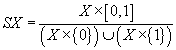
SX= (X x [0, 1])/((X x {0}) ∪ (X x {1}))

The n-th interation of taking the suspension is written SⁿX, and you define

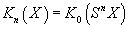
K_n(X) = K₀(SⁿX)

Bott periodicity says that K_n(X) is isomorphic to K_{n + 2}(X).

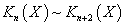
K_n(X) ~ K_{n + 2}(X)

If you had used real vector bundles instead of complex, you’d have periodicity of 8 instead of 2.

Often you would want to do away from topological spaces and replace them with their algebraic equivalent which is C*-algebras. Given the C*-algebra A = C(X) = {f : X → C} of continuous complex-valued functions on X, a vector bundle over X can equivalently be characterized as a projection in M_n(A), such as an n x n matrix P with values in A that satisfy P = P* = P². So an alternative way to define K₀, but now generalized to arbitrary C*-algebras A, is an abelian group K₀(A) which has one generator [P] for every projector in M_n.(A) for all n subject to the identification of projections which can be continuously connected and to the relation

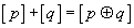
[p] + [q] = [p ⊕ q]

This formulation makes it easy to define a sort of dual K-theory. For every C*-algebra A, there is a dual C*-algebra Dρ(A) defined as the commutant up to compact operators of any representation of A. So given A, choose any representation ρ : A → B(H) of A in terms of bounded operators on some separable Hilbert space H, then

Dρ(A) = {T ∈ B(H) : [T, ρ(a)] ~0, for all a ∈ A}

Where T₁ ~T₂ means that T₁ – T₂ ∈ K(H) is a compact operator.

It may be that A didn’t have a unit. Let the result of making it unital by adjoining a unit be denoted [A tilde]. The K-theory of D([A tilde]) for any ρ is now called K-homology, and you write

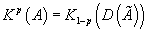
The position of the indices indicates where the maps are covariant and contravariant, when these are regarded as functors from the category of C*-algebras to that of abelian groups. The reason for calling the map A → K^p(A) a homology is that in the case where A = C(X) is the C*-algebra of functors on X, this map can be shown to define what is called a generalized homology theory. This is any theory that associates a list of groups to any topological space such that a couple of crucial properties from simplicial homology are satisfied. What is the homology theory corresponding to K^p? It turns out this is just the K-theory that we started with

K^p(A) ~Hom(K_p(A), Z)

K^p(C(X)) is nothing but equivalence classes of generalized Dirac operators on rank-p vector bundles over X.

A Fredholm operator is a bounded operator F which admits the idea of an index.

Index(F) = Dim(Kernel(F)) – Dim(Cokernel(F))

A Fredholm module is like a spectral triple with a Fredholm operator instead of a Dirac operator. Specifically, it’s a triple (H, ρ(A), F) of a Hilbert space H on which F and the C*-algebra A are represented by ρ : A → B(H). If in addition, a Clifford algebra Cp is represented by H which commutes with F, this is called a p-multigraded Fredholm operator.

Kasparov defined the Kasparov K-homology group KK^-p(A) to be the abelian group of equivalence classes of Fredholm modules. More precisely, KK^-p(A) is the abelian group generated by p-multigraded Fredholm modules (H, ρ(A), F) up to unitary equivalence, and are modules which can be continuously connected by the relation

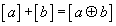
[a] + [b] = [a [direct sum] b]

where a and b are Fredholm operators, and [a] and [b] are their images in KK^-1(X). It turns out that Kasparov groups are isomorphic to ordinary K-homology groups.

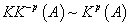
KK^-p(A) ~ K^p(A)

This gives an interpretation for the pairing between K-homology and K-theory.

The Atiyah-Singer index theorem is an important unifying result that connects topology and analysis. It deals with elliptic differential operators, such as the Laplacian, on compact manifolds. The index theorem, for instance, proves the impossibility of M. C. Escher’s “Ascending and Descending” where people, always climbing stairs, still manage to encircle the courtyard. We start with a compact manifold M, without boundary, a vector bundle E on M, and elliptic operator D over M. Here D is a differential operator acting on smooth sections of the vector bundle. The property of being elliptic is expressed by s which can be viewed as coming from the coefficients of the highest order part in D. The symbol s is defined on a vector bundle, the cotangent bundle, or phase space. The symbol s assigns to every point of the cotangent bundle a homeomorphism of E, meaning at each point in the cotangent bundle, E is a vector space, and s is a matrix acting on that vector space. Ellipticity is the requirement that s be invertible away from the zero section. The differential operator D gives rise to a Fredholm operator. Such a Fredholm operator has an index, defined as the difference between the dimension of the kernel of D, which are solutions of Df = 0, the harmonic functions, and the dimension of the cokernel of D, which are constraints on the right hand side on an inhomogeneous equation such as Df = g. The index problem is to compute the index D using only the symbol s and topological data derived from the manifold and vector bundle. The index theorem solves this problem using K-theory.

Now I’ll discuss the Thom isomorphism theorem. Let ξ → X be a d-dimensional vector bundle over a topological space X, and let h⁺ be a multiplicative generalized cohomology theory. Let

τ ∈ h^d(D(ξ), S(ξ))

be a Thom class for ξ where D(ξ) is the disk bundle of ξ, and S(ξ) is the sphere bundle of ξ. Since h⁺ is a multiplicative theory, there is a generalized cup product map

h*(D(ξ)) [direct product]_h*h*(D(ξ), S(ξ)) → h*(D(ξ), S(ξ))

where the tensor product is over the coefficient ring h*(pt) of the theory. Using the isomorphism

p* : h⁺(X) ~h*(D(ξ))

induced by the homotopy equivalence p : D(ξ) → X we get the homeomorphism

T: hⁿ(X) → h^{n x d}(D(ξ), S(ξ)) ~ [h tilde]^{n + d}(X^ξ)

Taking α to p*(α) . τ. And where X^ξ is the Thom space D(ξ)/S(ξ) of ξ. The Thom isomorphism theorem then says T is an isomorphism

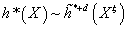
h*(X) ~[h tilde]*^{+ d}(X^ξ)

of graded modules over h*(pt).

There’s one last subject I have to discuss before we begin. A character class is a way of associating to each principle bundle on a topological space X, a cohomology class of X. The cohomology class measures the extent to which the bundle is twisted, especially whether it contains sections or not. Therefore, characteristic classes are global invariants which measure the deviation of a local product structure from a global product structure.

If G is a topological group for a topological space X, then b_G(X) is the set of isomorphism classes of principle G-bundles. b_G(X) is a contravariant functor from the category of topological spaces and continuous functions to the category of sets and functions, or Top → Set, sending a map f to the pull back operation f*. A characteristic class c of principle G-bundles is then a natural transformation from b_G(X) to a cohomology functor H*, which is also a functor to Set. Therefore, the characteristic class c is a transformation from one functor to another. A characteristic class associates to any principle G-bundle P → X an element c(P) in H*(X) such that if f : Y → X is a continuous map, then c(f*P) = f*c(P). On the left is the class of the pull back of P to Y. On the right is the image of the class of P under the induced map in cohomology.

Characteristic classes are contravariant constructions, thus belonging to cohomology theory in that a section is a kind of function on space. Cohomology was developed after homology and homotopy which are covariant theories mapping into space. Characteristic classes were first considered in the 1930s, and they were a major reason why a dual theory to homology was sought. The characteristic class approach to curvature invariants was one of the primary motivations to developing cohomology, in order to prove the Gauss-Bonnet theorem. When the theory was organized around 1950, it became clear that the most fundamental characteristic classes known at the time, which were the Chern class, the Pontryagin class, and the Stiefel-Whitney class, were reflections of the classical linear groups and their maximal torus structure. It was realized that the Chern class had been foreshadowed by the Schubert calculus on Grassmannians, and the Italian school of algebraic geometry. However, now there was a framework which produced families of classes whenever there was a vector bundle involved.

Given a space X carrying a vector bundle, that implied in the homotopy category, a mapping from X to a classifying space BG, for the relevant linear group in G. For homotopy theory, the relevant information is carried by the compact subgroups, such as the orthogonal groups and the unitary groups of G. Once the cohomology H*(BG) was calculated, the contravariant property of cohomology meant that the characteristic classes for the bundle would be defined in H*(X) in the same dimensions. For example, the Chern class is really one class with graded components in each even dimension. With the advent of extraordinary cohomology theory, when K-theory and cobordism theory were developed in 1955, it was really only necessary to change the letter H everywhere to say what the characteristic classes were.

Chern classes, pronounced “Chen”, were invented by Shiing-Shen Chen in 1940. A chern class is a gadget defined for complex vector bundles. The Chern classes of a complex manifold are the Chern classes of its tangent bundle. The ith Chern class is an obstruction to the existence of an (n – i + 1) everywhere complex linearly independent vector fields on that vector bundle. The ith Chern class is in the (2i)-th cohomology group of the base space.

Chern classes are topological invariants associated to vector bundles on a smooth manifold. If you describe the same vector bundle on a manifold in two different ways, the Chern classes will be the same. How can you tell if two vector bundles are the same? If the Chern classes of two vector bundles are different then the vector bundles must be different, although if they are the same, it doesn’t mean that the vector bundles are the same. It is often important to count how many linearly independent sections a vector bundle has. The Chern classes offer some information about this, such as through the Riemann-Roch theorem and the Atiyah-Singer index theorem. Chern classes are also easy to calculate since they can be expressed as polynomials of coefficients of the curvature form.

Given a complex hermitian vector bundle V of complex rank n over a smooth manifold M, a representative of each Chern class, also called a Cern form, c_k(V) of V, are given as the coefficients of the characteristic polynomial of the curvature form Ω of V.

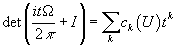
det((itΩ/2π) + I) = [summation over k] c_k(V)t^k

where Ω is the curvature form, the scalar t is an indeterminate to generate the sum from the determinate, and I is the n x n identity matrix.

The determinant is over the ring of n x n matrices whose entries are polynomials in t with coefficients in the commutative algebra of even differential forms on M. The curvature form Ω of V is defined as

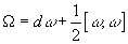
Ω = dω + ½ [ω, ω]

where ω is the connection, and d is the exterior derivative, or via the same expression in which ω is a gauge form for the gauge group V.

When you say “Chern class”, you mean “class up to addition of a differential form”. Therefore, Chern classes are cohomology classes in the sense of de Rham cohomology. It can be shown that the cohomology class of the Chern forms do not depend on the choice of connection in V.

If you ever look at a little girl in pigtails, you see they have a vertical line down the back of their head. If you try combing the hair of a child, you see there are lines where on one side, the hairs point in one direction, and on the other side, the hairs point in the other direction. Let’s say you have a vector field on a sphere.

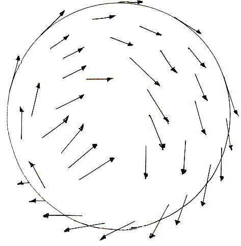
Is it possible to arrange the vectors in such a way so there is no point on the sphere where they suddenly change direction? The answer to the question is “no”. This is called the hairy ball theorem, which states you can’t comb a hairy ball flat. This fact can be proved using Chern classes.

Let’s say you have one-dimensional complex projective space, CP¹, also called a Riemann sphere. Let’s say z is a holomorphic local coordinate for the Riemann sphere. Let V = TCP¹ be the bundle of complex tangent vectors having the form a ∂/∂z at each point, where a is a complex number. You can prove that V has no section that is everywhere nonzero, proving the complex version of the hairy ball theorem.

The first Chern class of a trivial bundle is zero.

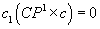
c₁(CP¹ x C) = 0

We need to show that

c₁(V) ≠ 0

If you have the Kahler metric

h = (dz d[z bar]/(1 + | z |²)

The curvature z-form is given by

Ω = (2dz ∧ d[z bar])/(1 + | z |²)²

The definition of the first Chern class is

c₁ = (i/2π)Ω

You compute its integral over the Riemann sphere.

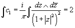
[integral]c₁ = (i/π) [integral] (dz ∧ d[z bar])/(1 + | z |²)²

after switching to polar coordinates. By Stokes theorem, an exact form would integrate to 0, so the cohomology class is non-zero. This proves that TCP¹ is not a trivial vector bundle, proving the complex version of the hairy ball theorem.

Given a complex vector bundle V over a topological space X, the Chern classes of V are a sequence of elements of the cohomology of X. The kth Chern class of V, written c_k(V) is an element of

H^2k(X ; Z)

The cohomology of X with integer coefficients. You can also define the total Chern class as

c(V) = c₀(V) + c₁(V) + c₂(V) + …

The Chern classes obey the following four axioms.

1. c₀(V) = 1 for all V

2. Functorality : If f : Y → X is continuous, and f*V is the vector bundle pull back of V, then c_k(f*V) = f*c_k(V).

3. Whitney sum formula: If W → X is another complex vector bundle, then the Chern classes of the direct sum V + W are given by

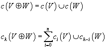
c(V + W) = c(V) ∪ c(W)

c_k(V + W) = [summation of i from 0 to n]c_i(V) ∪ c_{k – i}

4. Normalization : The total Chern class of the tautological line bundle over CP^k is 1 – H, where H is the Poincare dual to the hyperplane CP^{k – 1} ⊂ CP^k.

Alexander Grothendieck managed to replace these with the following three axioms.

1. Functorality : If f : Y → X is continuous, and f*V is the vector bundle pull back of V, then c_k(f*V) = f*c_k(V).

2. Additivity : If 0 → E → E’ → E” → 0 is an exact sequence of vector bundles, then c(E) = c(E’) = c(E”).

3. Normalization : If E is a line bundle, then c(E) = 1 + e(E_R, where e(E_R) is the Euler class of the underlying real vector bundle.

These properties uniquely uniquely characterize the Chern classes. They imply

1. If n is the complex rank of V, then c_k(V) = 0 for all k > n. This the total Chern class terminates.

2. The top Chern class of V, meaning c_n(V) where n is the rank of V, is always equal to the Euler class of the underlying real vector bundle.

A Calabi-Yau manifold is a Kahler manifold with vanishing first Chern class. A Calabi-Yau manifold of complex dimension n is called a Calabi-Yau n-fold. In 1957, Eugenie Calabi conjectured that all such manifolds admit a Ricci-flat metric, one in each Kahler class, and this was proved by Sing-Tung Yau in 1977. A Calabi-Yau n-fold is a manifold with SU(n) holonomy. The first Chern class vanishes if and only if the canonical bundle is trivial, which is the case if and only if the canonical bundle is the zero class. Here is a 3D slice of a 6D Calabi-Yau manifold used in superstring theory.

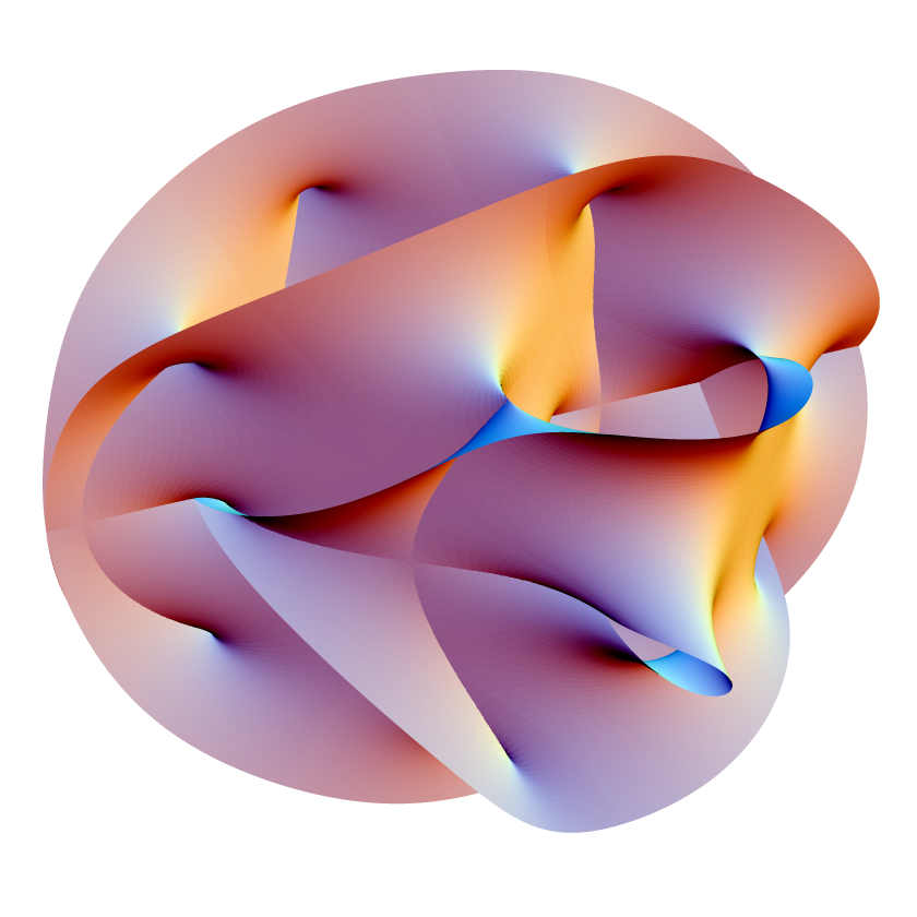
Aside from the Chern class, another characteristic class is the Pontryagin class. The ith Pontryagin class of a vector bundle is (-1)ⁱ times the ith Chern class of the complexification of the vector bundle. It is also the 4ith cohomology group of the base space involved.

Given a vector bundle E over M, its k-th Pontryagin class p_k(E) is defined as

p_k(E) = p_k(E, Z) = (-1)^kc_2k(E [direct product] C) ∈ H^4k(M, Z)

where

c_2k(E [direct product] C)

is times the 2k-th Chern class of the complexification

E x C = E + iE

Of E and H^4k(M, Z), the 4k-th cohomology group of M with rational coefficients.

Pontryagin classes have a meaning in real differential geometry, as opposed to the Chern class which assumes a complex vector bundle.

If all Pontryagin classes and Stiefel-Whitney classes of E vanish, then the bundle is trivial. Its Whitney sum with a trivial bundle is trivial. The total Pontryagin class

p(E) = 1 + p₁(E) + p₂(E) + … ∈ H*(M, Z)

is multiplicative with respect to the Whitney sum of vector bundles.

p(E + F) = p(E) ∪ p(E)

for two vector bundles E and F over M

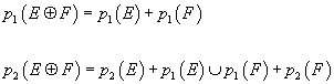
p₁(E + F) = p₁ + p₁(F)

p₂(E + F) = p₂(E) + p₁(E) ∪ p₁(F) + p₂(F)

Given a 2k-dimensional vector bundle E you have

p_k(E) = e(E) ∪ e(E)

where e(E) is the Euler class of E, and ∪ is the cup product of cohomology classes.

In 1948, Shiing-Shen Chern and Andre Weil proved that the rational Pontryagin classes

p_k(E, Q) ∈ H^4k(M, Q)

can be presented as differential forms which depend polynomially on the curvature form of a vector bundle. This Chern-Weil theory revealed a major connection between algebraic topology and global differential geometry.

For a vector bundle E over an n-dimensional differentiable manifold M equipped with a connection, its k-th Pontryagin class can be realized by the 4k-form

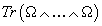
Tr(Ω ∧ …∧ Ω)

constructed with 2k copies of the curvature form Ω. The value

p_k(E, Q) = [Tr(Ω ∧ …∧ Ω)] ∈ H_dR^4k(M)

does not depend on the choice of connection. H*_dR(M) is the de Rham cohomology groups.

The third main type of character class, after the Chern class and Pontryagin class, is the Stiefel-Whitney class. The ith Stiefel-Whitney class of a real vector bundle, or tangent bundle on a real manifold, is in the ith cohomology group of the base space involved. It is an obstruction to the existence of (n – i + 1) real linearly independent vector fields on that vector bundle, where n is the dimension of the fiber. Here “obstruction” means that the ith Stiefel-Whitney class being nonzero implies that there do not exist (n – i + 1) everywhere linearly dependent vector fields, although the Stiefel-Whitney classes are not always the obstruction. In particular, the nth Stiefel-Whitney class is the obstruction to the existence of an everywhere nonzero vector field, and the first Stiefel-Whitney class of a manifold is the obstruction to orientability.

Stiefel-Whitney classes are a type of characteristic class associated to real vector bundles E → X. They are written w_i(E) taking values in Hⁱ(X, Z₂), the cohomology groups with mod 2 coefficients. For example, over the circle, S¹, there is a line bundle that is topologically non-trivial, that is the line bundle associated with the Möbius strip, usually thought of as having fibers [0, 1]. The cohomology group

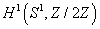
H¹(S¹, Z/2Z)

has just one element other than 0, which is the first Stiefel-Whitney class, w₁, of that line bundle.

Stiefel-Whitney classes obey the following four axioms.

1. For every real line bundle E → X, there exists w_i(E) in Hⁱ(X, Z/2Z) which are natural, in other words, f*w_i(E) = w_i(f*E) for any continuous map between spaces.

2. w₀(E) = 1 in H⁰(X; Z/2Z)

3. Normalization condition: w_i(γ¹) = x in H¹(RP¹; Z/2Z) = Z/2Z, where γⁿ is the canonical line bundle.

4. Whitney product formula:

w_k(E + F) = [summation over i + j = k] w_i(E) ∪ w_j(F)

The Chern classes can be used to construct a homomorphism of rings from the topological K-theory of a space to the completion of its rational cohomology. For line bundles V, the Chern character ch is defined by

ch(V) = exp(c₁(V))

For sums of line bundles, the Chern character is defined by addivity. For arbitrary vector bundles, it is defined by pretending that the bundle is a sum of line bundles. For sums of line bundles, the Chern character can be expressed in terms of Chern classes, and we use the same formulas to define it on all vector bundles. For example, the first few terms are

ch(V) = dim(V) + c₁ + c₁(V)²/2 – c₂(V) + …

If V is filtered by line bundles L₁, L₂,…L_k having first Chern classes x₁, x₂,…x_k respectively, then

ch(V) = e^x₁ + e^x₂ +…+e^x_k

If the connection is used to define the Chern classes, then the explicit form of the Chern character is

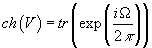
ch(V) = tr(exp(iΩ/2π))

where Ω is the curvature of the connection.

The Chern character is useful partly because you can use it to compute the Chern class of a tensor product. Specifically, it obeys

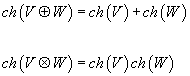
ch(V + W) = ch(V) + ch(W)

ch(V x W) = ch(V) ch(W)

Using the Grothendieck addivity axiom for Chern classes, the first of these identities can be generalized to a state where ch is a homomorphism of abelian groups from the K-theory K(X) into the rational cohomology of X. The second identity establishes the fact that this homomorphism also respects products in K(X), and so ch is a homomorphism of rings.

The Steenrod algebra has to do with the cohomology operations in singular cohomology with integer mod 2 coefficients. For every n ∈ Z, and i ∈ {0, 1, 2, 3,…}, there are natural transformations of functors

Sqⁱ : Hⁿ(X, Z₂) → H^{n + i}(X, Z₂)

satisfying the following axioms.

1. Sqⁱ = 0 for i > n

2. Sqⁿ(X) = X ∪ X for all X ∈ Hⁿ(X, A; Z₂) and all pairs (X, A)

3. Sq⁰ = id_{Hⁿ(X, Z2)}

4. The Sqⁱ maps commute with the coboundary maps in the long exact sequence of a pair. In other words

Sqⁱ : Hⁿ(X, Z₂) → H^{n + i}(X, Z₂)

is a degree i transformation of cohomology theories.

5. Cartan relations:

Sqⁱ(x ∪ y) = [summation over j + k = i] Sqⁱ (x) ∪ Sq^k(y)

6. Adem relations:

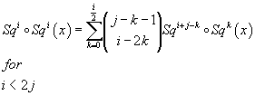
Sqⁱ o Sqⁱ(x) = [summation over k from 0 to i/2] (j – k – 1 i – 2k) Sq^{i + j – k} o Sq^k(x), for i < 2j

7.

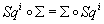
Sqⁱ o Σ = Σ o Sqⁱ

Where Σ is the cohomology suspension isomorphism.

The existence of these cohomology operations endows the cohomology ring with the structure of a module over the Steenrod algebra A, defined to be T(F_Z2 {Sqⁱ : i ∈ {0, 1, 2, 3,…}})/R where F_Z2(x) is the free module functor that takes any set, and sends it to the free Z₂ module over that set. We think of F_Z2 {Sqⁱ : i ∈ {0, 1, 2, 3,…}} as being a graded Z₂ module, where the ith gradation is given by Z₂ . Sqⁱ. This makes the tensor algebra T(F_Z2 {Sqⁱ : i ∈ {0, 1, 2, 3,…}}) into a graded algebra over Z₂. R is the ideal generated by the elements

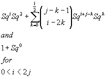
Sqⁱ Sq² + [summation over k from 0 to i/2] Sq^{i + j – k} Sq^k and 1 + Sq⁰ for 0 < i < 2j

This makes A into a graded Z₂ algebra.

By the definition of the Steenrod algebra, for any space (X, A), Hⁿ(X, A; Z₂) is a module over the Steenrod algebra A, with multiplication induced by Sqⁱ . x = Sqⁱ(x). Therefore, cohomology with coefficients in the ring Z₂, Hⁿ(X, Z₂) is a functor from the category of pairs of topological spaces to graded modules over A.

Finally, we reach the point where we are able to start talking about what this paper is supposed to be about, which is the relation between K-theory and superstring theory. I assume the reader is already very familiar with superstring theory and M-theory. I assume that you have already read my previous paper “Beyond the Standard Model”. Of course, that paper is intended as an introduction to the subject. For more detail, I recommend Joseph Polchinski’s excellent textbooks “String Theory”, Volumes I and II. K-theory allows us to easily extract information about a manifold. In superstring theory, all of the details of the low energy physics, which is the world we see around us, such as the particle spectrum, etc., is determined by the details of the topology of the compact manifold that the extra dimensions are compactified on. Therefore, we can use K-theory to see what superstring theory actually predicts, and see if it matches the real world, Obviously, this is very important. Therefore, this very obscure branch of arcane mathematics has suddenly become extremely important for advanced physics. This increased interest in K-theory by physicists has in turn spurred further advancement in pure mathematics. There is a constant give and take between mathematics and physics, like a feedback mechanism. Throughout most of human history, for thousands of years, from Mesopotamia, Egypt, Greece and Rome, up to and including the present day, the needs of physics and astronomy have been the primary driving force behind the development of mathematics. Examples of physics and mathematics stimulating each other include Rene Descartes’ numerical model of space, Newton’s concept of differential equations, and James Clerk Maxwell’s vector field theory. Newton and Leibniz developed calculus to express Newtonian mechanics. Einstein’s discovery of general relativity suddenly increased the importance of Riemannian geometry. The fact that K-theory can be used to study superstring theory has increased our understanding of K-theory, which in turn has then increased our understanding of superstring theory.

In superstring theory, K-theory is conjectured to classify the allowed Ramond-Ramond field strengths, and also the charges of stable D-branes. This conjecture was first proposed in 1997 by Ruben Minasian and Gregory Moore in their paper “K-theory and Ramond-Ramond charge”. It was popularized by Edward Witten in his paper “D-branes and K-theory” where he demonstrated that in Type IIB string theory, it arises naturally from Ashoke Sen’s realization of arbitrary D-brane configurations as stacks of D9-branes and anti-D9-branes after tachyon condensation. Such stacks of branes are inconsistent in a non-torsion Neveu-Schwarz (NS) 3-form background which, as was pointed out by Anton Kaputsin, complicates the extension of K-theory classification to such cases. Peter Bouwknoght and Mathai Varghese suggested a solution to this problem. D-branes are in general classified by twisted K-theory which had been defined in 1989 by Jonathan Rosenberg.

The K-theory classification of D-branes has numerous applications. For instance, Amihay Hanany and Barak Kol used it to argue that there are eight species of orientifold one-plane. Angel Urganga applied the K-theory classification to derive new consistency conditions for flux compactification. K-theory has also been used to conjecture a formula for the topologies of T-dual manifolds. Recently, K-theory has been conjectured to classify the spinors in compactifications on generalized complex manifolds.

Despite these successes, RR fluxes are not quite classified by K-theory. In their paper “In E₈ Gauge Theory and a Derivation of K-theory from M-theory”, Emanuel Diaconescu, Gregory Moore, and Edward Witten (DMW) argued that the K-theory classification is incompatible with S-duality in Type IIB string theory. Another problem is that if you try to classify the fluxes on a compact ten-dimensional spacetime, then a complication arises due to the self-duality of the RR fluxes. The duality uses the Hodge star, which depends on the metric, and so is continuously valued, and thus usually irrational. Therefore, not all the RR fluxes, which are interpreted as Chern characters in K-theory, can be rational. However, Chern characters are always rational. You have to choose half the fluxes to quantize, or a polarization in the geometric quantization inspired language of DMW, and later Mathai Varghese and Hisham Sati. You could also use the K-theory of a 9-dimensional time slice, as was done by Juan Maldacena and Nathan Seiberg.

In the classical limit of Type II string theory, which is Type II supergravity, the Ramond-Ramond field strengths are differential forms. In the quantum theory, the well-definedness of the partition functions of D-branes implies that the RR field strengths obey Dirac quantization conditions when spacetime is compact, or when a spatial slice is compact, and you consider only the magnetic components of the field strength which lies along the spatial directions. This led 20th Century physicists to classify RR field strengths using cohomology with integer coefficients.

However, some authors have argued that the cohomology of spacetime with integer coefficients is too large. For example, in the presence of Neveu-Schwarz H-flux or non-spin cycles, some RR fluxes dictate the presence of D-branes. In the former case, this is a consequence of the supergravity equation of motion which states that the product of an RR-flux with the NS 3-form is a D-brane charge density. Thus the set of topologically distinct RR field strengths that can exist in brane-free configurations is only a subset of the cohomology with integer coefficients. This subset is still too big because some of these classes are related by gauge transformations. In QED, there are gauge transformations which add integer multiples of 2π to Wilson loops. The p-form potentials in Type II supergravity theories also have these large gauge transformations but due to the presence of Chern-Simon terms in supergravity actions, these gauge transformations transform not only the p-form potentials but also the (p + 3)-form field strengths. Thus to obtain the space of inequivalent field strengths from the subset of integral cohomology, we must quotient these by the gauge transformations.

The Atiyah-Hirzebruch spectral sequence constructs twisted K-theory, with the twist given by the NS 3-form field strength, as a quotient of a subset of the cohomology with integer coefficients. In the classical limit, which corresponds to working with rational coefficients, this is precisely the quotient of the subset described above with supergravity. The quantum corrections come from torsion classes and contain mod 2 torsion corrections due to the Freed-Witten anomaly.

Twisted K-theory classifies the subset of RR field strengths that can exist in the absence of D-branes quotiented by large gauge transformations. Daniel Freed has attempted to extend this classification to include the RR potentials using differential K-theory.

K-theory classifies D-branes in noncompact spacetimes, intuitively in spacetimes in which we are not concerned about the flux sourced by the brane having nowhere to go. While the K-theory of a 10d spacetime classifies D-branes as a subset of that spacetime, if the spacetime is the product of time and a fixed 9-manifold, then K-theory also classifies the conserved D-brane charges on each 9-dimensional spatial slice. While we are required to forget about the RR potentials to obtain the K-theory classification of RR field strengths, we are required to forget about the RR field strengths to get the K-theory classification of D-branes.

Petr Horava pointed out that K-theory classification of D-branes is independent of, and in some ways stronger than, the classification of BPS states. K-theory appears to classify stable D-branes that are missed by supersymmetry based classifications. For example, D-branes with torsion charges, meaning charges in the order N cyclic group Z_N, attract each other, and so can never be BPS. In fact, N such D-branes can decay, while no superposition of branes that satisfy a Bogomolny bound can ever decay. However, the charge of such branes is conserved modulo N, and this is captured by the K-theory classification but not a BPS classification. Such torsion branes have been applied, for example, to model Douglas-Shenker strings in supersymmetric U(N) gauge theories.

Ashoke Sen has conjectured that in the absence of a topologically nontrivial NS 3-form, all Type IIB brane configurations can be obtained from stacks of space filling D9 and anti-D9 branes via tachyon condensation. The topology of the resulting branes is encoded in the topology of the resulting gauge bundle on the stack of the space filling branes. The topology of the gauge bundle on a stack of D9s and anti-D9s can be decomposed into a gauge bundle on the D9s, and another gauge bundle on the anti-D9s. Tachyon condensation transforms such a pair of bundles into another pair in which the same bundle is direct summed with each component of the pair. Thus the tachyon condensation invariant quantity, which is the charge which is conserved in the tachyon condensation process, is not a pair of bundles but is instead an equivalence class of a pair of bundles under the direct sum of the same bundle on both sides of the pair. This is precisely the usual construction of topological K-theory. Thus the gauge bundles on stacks of D9s and anti-D9s are classified by topological K-theory. According to Sen’s conjecture, all D-brane configurations in Type IIB are then classified by K-theory. Petr Horova has extended this extended this conjecture to Type IIA using D8-branes.

While the tachyon condensation picture of K-theory classification classifies D-branes as subsets of a 10-dimensional spacetime with no NS 3-form flux, the Maldacena, Moore, Seiberg picture classifies stable D-branes with finite mass as subsets of a 9-dimensional spatial slice of spacetime. The main point is that D-branes are not classified by integral cohomology because Dp-branes wrapping certain cycles suffer from a Freed-Witten anomaly which is cancelled by the insertion of D(p – 2)-branes, and sometimes D(p – 4)-branes, that end on the Dp-brane. These inserted branes may either continue to infinity, in which case the composite object has infinite mass, or they may end on an anti-Dp-brane, in which case the total Dp-brane charge is zero. In either case, you would probably want to remove the anomalous Dp-branes from the spectrum leaving only a subset of the original integral cohomology. The inserted branes are unstable. To see this, imagine that they extend in time into the past, away from the anomalous brane. This corresponds to a process in which the inserted branes decay via a Dp-brane that forms, wraps around the cycle, and then disappears. Maldacena, Moore, and Seiberg refer to this process as an instanton, although it doesn’t have to be instantonic. The conserved charges are thus the nonanomalous subset quotiented by the unstable insertions. This is precisely the Atiyah-Hirzebruch spectral sequence construction of twisted K-theory as a set.

Diaconescu, Moore, and Witten (DMW), have pointed out that the twisted K-theory classification is not compatible with S-duality covariance in Type IIB string theory. For example, here you have the 3-form field strength G₃ in the Atiyah-Hirzebruch spectral sequence (AHSS)

d₃G₃ = Sq³G₃ + H ∪ G₃ = G₃ ∪ G₃ + H ∪ G₃ = 0

where d₃ = Sq³ + H is the first nontrivial differential in the AHSS, Sq³ is the third Steenrod square, and the last equality follows from the fact that the n-th Steenrod square acting on any n-form x is x ∪ x. The above equation is not invariant under S-duality which exchanges G₃ and H. Instead, DMW have proposed the following S-duality covariant extension

G₃ ∪ G₃ + H ∪ G₃ + H ∪ H = F

Where F is an unknown characteristic class that depends only on the topology, and not on the fluxes. Diaconescu, Freed, and Moore wrote a paper titled, “The M-theory 3-form and E₈ Gauge Theory” in which they found a constraint on F using the E₈ gauge theory approach to M-theory pioneered by DMW. Thus D-branes in Type IIB are not classified by twisted K-theory after all, but by some unknown S-duality covariant object that also classifies both fundamental strings and NS5-branes.

The method of calculating twisted K-theory invented by Maldacena, Moore, and Seiberg (MMS) can also easily S-covariantized since the Freed-Witten anomalies respect S-duality. Thus the S-covariantized form of the MMS construction can be applied to construct the S-covariantized twisted K-theory, as a set, without knowing what the S-covariantized object is. This program has been carried out in a number of papers, and has been applied to fluxes, and has been used to prove DMW’s conjectured constraint on 3-fluxes, and they show there is an additional term equal to the D-brane charge. The Klebanov-Strassler cascade of Seiberg dualities consists of a series of S-dual MMS instantons, one for each Seiberg duality. The group Z_N of universal classes of the SU(M + N) x SU(M) supersymmetric gauge theory is then shown to agree with the S-dual twisted K-theory, and not with the twisted K-theory.

So basically, we started with K-theory, and because the cohomology of spacetime with integer coefficients was too large, we moved to twisted K-theory, and then because it was inconsistent with S-duality in Type IIB theory, we moved to S-covariantized twisted K-theory. Hisham Sati and Igor Kriz propose that instead of using any type of twisted K-theory at all, we should instead classify Type II string theory configurations using elliptic cohomology.

Let me illustrate how to apply some of the ideas we’ve discussed to string theory. Let’s say you have Type I string theory on R¹⁰. Let’s look at the following homotopy group of SO(32).

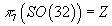
π₇(SO(32)) = Z

SO(32) bundles on the (i + 1)-dimensional sphere S^{i + 1} are classified by π_i(SO(32)). SO(32) bundles on S^{i + 1} are equivalent to SO(32) bundles on Euclidean space R^{I + 1} that are trivialized at infinity, meaning that the pure gauge at infinity and the action integral on R^{i + 1} converges. So you can use π₇ to construct strings.

The string associated with π₇(SO(32)), called a gauge string, can be identified as follows. Let B be the two-form field of Type I superstring theory. It is a Ramond-Ramond field and couples to the D-string. However, B also couples to the gauge string because of the Green-Schwarz anomaly canceling term

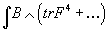
∫ B ∧ (tr F⁴ + …)

since the gauge string is made from a gauge field on R⁸ with nonzero integral

∫_R⁸ (tr F⁴ + …)

The minimal gauge string has D-string charge ±1. This suggests that the string constructed in low energy field theory using a generator of π₇(SO(32)) shrinks dynamically to an ordinary D-string.

To compute the D-string charge of the gauge string, let V be an SO(32) bundle on R⁸ with a connection of finite action. Because the connection is flat at infinity, we can compactify and regard V as an SO(32) bundle on S⁸. This bundle has first Pontryagin class p₁(V) = 0 since p₁(V) would take values in H⁴(S⁸) which vanishes and

∫_S⁸ p₂(V) = 6k

where k is an arbitrary integer. The factor of 6 arises as follows. The topological charge of an SO(32) bundle V on S⁸ is measured by the Dirac index, which, depending on the choice of V, can be an arbitrary integer k. However, using the index theorem, the Dirac index for spinors on S⁸ valued in V is

[integral over S⁸] ch(V) = [summation over i] [integral over S⁸] (e^λ_i + e^-λ_i) = -[integral over S⁸] p₂(V)/6

where λ_i are the roots of the Chern polynomial, the Pontryagin classes are

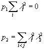
p₁ [summation over i] λ_i² = 0

p₂ = [summation over i < j] λ₁² λ₂²

and ch is the Chern character. Therefore p₂(V) can be any multiple of 6.

At the same time, the standard anomaly twelve-form, which is the one loop anomaly of the massless gravitinos and gluinos of the Type I theory, is

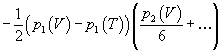
-½(p₁(V) – p₁(T))(p₂(V)/6 +… )

Since the field strength H of the B-field, normalized so that the periods of B are multiples of 2π,obeys

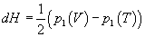
dH = ½(p₁(V) – p₁(T))

the properly normalized coupling of B to p₂(V) is

∫ B ∧ p₂(V)/6

since p₂(V)/6 can be any integer, it follows that the minimal gauge string has D-string charge 1, and thus can be identified with the D-string.

In string theory, you are often concerned with the stability of D-branes and this has to do with how D-branes can wrap around the compactified dimensions, called cycles, and also the charges of the D-branes, such as the Neveu-Schwarz charge H, or Ramond-Ramond charge F. Also, you have to consider the possibility that a brane and antibrane could annihilate. Let’s say, with Type II string theory, you have a p-brane and an anti-p-brane, written [p bar]-brane, both wrapped around the same submanifold W of a spacetime X. In this case, the p-brane and anti-p-brane could annihilate. You have open strings with both ends on the p-brane, called p-p strings, open strings with one end on the p-brane and the other end on the anti-p-brane, called p-[p bar] strings, and finally open strings with both ends on the anti-p-brane, called [p bar]-[p bar] strings. The p-p open string spectrum consists of a massless super-Maxwell multiplet plus massive excitations. The familiar NS sector tachyon is removed by the GSO projection. The [p bar]-[p bar] open strings give another super-Maxwell multiplet. However, for p-[p bar] and [p bar]-p open strings, you have to make the opposite GSO projection. Therefore, the massless vector multiplet is projected out, and the tachyon survives. The fact that you are left with a tachyon after GSO projection means that the system is unstable, and what that means is that the brane and antibrane would annihilate each other. The instability associated with the tachyon represents a flow towards annihilation of the brane-antibrane pair. By giving the tachyon field a suitable excitation value, you can return to the vacuum state without the brane-antibrane pair.

The gauge group on the brane-antibrane pair is U(1) x U(1), with one U(1) on the brane, and the other U(1) on the antibrane. The tachyon field T has charges (1, -1), and its expectation value breaks U(1) x U(1) to a diagonal U(1) subgroup. This U(1) must ultimately be eliminated in the brane-antibrane annihilation.

The fact that the p-[p bar] and [p bar]-p strings have a reversed GSO projection can be explained as follows. Let’s say you have a p-[p bar] brane system, and it has a Chan-Paton label i, where i = 1 for an open string ending on a p-brane, and i = 2 for an open string ending on a [p bar]-brane. So therefore, you have an open string, and at each end of the open string, you have a charge that takes values in a two-dimensional Hilbert space. Let’s say the i = 1 state is bosonic, and the i = 2 state is fermionic. Then the GSO operator, (-1)^F, which usually acts trivially on the Chan-Paton factors, here acts by

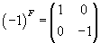
The p-p and [p bar]-[p bar] open strings have diagonal Chan-Paton wavefunctions. The wavefunctions are even under (-1)^F, leading to the usual GSO projection on the oscillator modes. The Chan-Paton wavefunctions for the p-[p bar] and [p bar]-p open strings are off-diagonal, and odd under (-1)^F, leading to a reversed GSO projection. If you were to multiply the above equation by an overall factor of -1, in the action of (-1)^F on string states, it would cancel out since each open string has two ends.

Having one bosonic and one fermionic Chan-Paton state would lead, if we made no GSO projection, to a gauge supergroup U(1|1). Because of the GSO projection, the off-diagonal fermionic gauge fields of U(1|1) are absent, so we instead get a structure whose lowest modes correspond to a superconnection, which is a matrix of the form

where A and A’ are the gauge fields, and T is the p-[p bar] tachyon. If E and F are bundles of bosonic and fermionic Chan-Paton states respectively, and A and A’ are connections on E and F, then T is a section of E ⊗ F*, and [T bar] is a section of E* ⊗ F, where E* is the dual of the bundle of E.

Now let’s consider a more general case with n p-branes and n [p bar]-branes wrapped on the submanifold W of spacetime. We allow an arbitrary U(n) gauge bundle E for the p-branes, and topologically the same bundle for the [p bar]-branes. The reason for having the same gauge bundle for both branes and antibranes is to make sure the overall system carries no D-brane charge. The operator (-1)^F_L maps p-branes to [p bar]-branes, and reverses the sign of all D-brane charges, while leaving fixed the gauge fields on the branes. Since there is no conserved charge, there is a tachyon field in the p-[p bar] sector, and you would expect any such system of branes to annihilate.

Now, let’s first specialize to the case of Type IIB superstrings, and secondly, we will use only 9-branes and anti-9-branes. We start with an arbitrary number of n 9-branes, and the same number of anti-9-branes. The reason we require the same number of 9-branes and anti-9-branes is so we have tadpole cancellation. In general, the 9-branes carry a U(n) gauge bundle E, and the [9 bar]-branes carry a U(n) gauge bundle F. We will label this configuration by the pair (E, F). What other configurations (E’, F’) is the configuration (E, F) equivalent to? The basic equivalence relation is brane-antibrane creation and annihilation. Any collection of m 9-branes and m [9 bar]-branes, with the same U(m) gauge bundle H for both branes and antibranes, can be created and annihilated. So the pair (E, F) can be smoothly deformed to

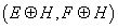
(E ⊕ H, F ⊕ H)

Since we are only interested in keeping track of conserved D-brane charges, properties that are invariant under smooth deformations, we consider the pair (E, F) to be equivalent to

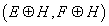
(E ⊕ H, F ⊕ H)

What we have arrived at is the definition of the K-group K(X), which is defined by saying that an element of K(X) is a pair of complex vector bundles (E, F) over spacetime, subject to an equivalence relation which is generated by saying that (E, F) is equivalent to (E ⊕ H, F ⊕ H) for any H. K(X) is a group, the sum of (E, F) and (E’, F’) being

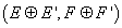
(E ⊕ E’, F ⊕ F’)

It’s actually a ring with the product of (E, F) and (E’, F’) being

(E ⊗ E’ ⊕ F ⊗ F’, E ⊗ F’ ⊕ F ⊗ E’)

as if the E’s were bosonic, and the F’s fermionic.

(E, F) can be written E – F. The subgroup of K(X) consisting of elements such that E and F have the same rank, meaning having equal numbers of 9-branres and [9 bar]-branes, is usually called [K tilde](X).

Therefore, tadpole canceling 9-[9 bar] configurations, modulo creation and annihilation of brane-antibrane pairs, are classified by [K tilde](X).

The spacetime X is usually noncompact, such as X = R⁴ x M, where M is compact. Because of a finite action or finite energy restriction, you want objects that are equivalent to the vacuum at infinity. This means that near infinity, you can relax to the vacuum by tachyon condensation. If there are no branes in the vacuum, then in the pair (E, F), E is isomorphic to F.

In general, the vacuum may contain branes, and this may be represented by a nonzero K-theory class. Tadpole cancellation, meaning that the condition that the equations of motion of Ramond-Ramond fields should have solutions, typically determines the K-theory class of the vacuum in terms of K-theory data. Requiring that the class (E, F) is equivalent to the vacuum, we get a K-theory class (E’, F’) that is trivial at infinity, in the sense that E’ and F’ are isomorphic at infinity. The Ramond-Ramond charge of an excitation of a given vacuum is best measured by subtracting the K-theory class of the vacuum from its K-theory class. Therefore in the most physical applications, the Ramond-Ramond charge of an excitation of the vacuum is considered to take values not in the ordinary K-group K(X) but in K-theory with compact support. A K-theory class with compact support is always represented by a pair of bundles of equal rank, since bundles that are isomorphic at infinity have equal rank. Therefore, the distinction between K(X) and [K tilde](X) is not important for most physical applications.

Up until now, we’ve been discussing Type IIB theory. Let’s now address Type I and Type IIA. For Type I theory, let’s say you have a system of n 9-branes, and m [9 bar]-branes. Tadpole cancellation says that n – m = 32. The branes support an SO(n) bundle E and an SO(m) bundle F. By brane-antibrane creation and annihilation, we assume that the pair (E, F) is equivalent to (E ⊕ H, F ⊕ H) for any SO(k) bundle H. Pairs (E, F) with this equivalence relation define the real K-group of spacetime, written KO(X). The subgroup with n – m = 0 is called [KO tilde](X). Any configuration with n – m = 32 can be naturally mapped to [KO tilde](X) by adding to F a rank 32 trivial bundle. Therefore, pairs (E, F) subject to the equivalence relation, and with n – m = 32, are classified by [KO tilde](X). You want to measure the K-theory class of an excitation relative to the vacuum, so then the brane charge of an excitation is measured by [KO tilde](X) with a compact support condition. If you have a compact support condition, KO(X) and {KO tilde](X) are equivalent, so you can say that 9-[9 bar] configurations in Type I are classified by KO(X). Unlike the situation in Type IIB, the identification of 9-brane configurations in Type I with KO-theory does not require assumptions about brane-antibrane annihilation. Since X has dimension 10, the classification of SO(32) bundles on X is governed by the homotopy groups π_i(SO(32)) for i ≤ (, and the relations between them. These homotopy groups are in the stable range, and the SO(32) bundles on X are classified by [KO tilde](X).

Now, I’ll briefly discuss Type IIA theory. Here you relate branes not to bundles on X but to bundles on X x S¹. This might be related to the circle used in relating Type IIA to M-theory. Given a p-brane wrapped on an odd-dimensional submanifold Z ⊂ X, we identify Z with a submanifold Z’= w x Z in X x S¹, where w is any point in S¹. Z’ has even codimension in X x S¹. A brane wrapped on Z’ determines an element of K(X x S¹). This element is trivial when restricted to X, meaning w’ x X for any w ∈ S¹. Two Type IIA brane configurations on X are equivalent if they determine the same element of K(X x S¹). The subgroup of K(X x S¹) consisting of elements that are trivial on X is called K'(X). By Bott periodicity, K(X) and K'(X) are the only complex K-groups of X. Therefore, we have two K-groups and two Type II string theories, so you have one K-group for each Type II string theory. For application to Type IIA, you need the subgroup [K tilde]'(X) = [K tilde](X x S¹) since we have no physical interpretation of 10-branes wrapping X x S¹. Therefore, D-brane charges in Type IIA are classified by K’(X) with an appropriate compact support condition.

Up until now, we’ve been talking about a stack of 9-branes and anti-9-branes. However, according to Sen’s conjecture, any p-brane with p ≤ 9 is equivalent to a stack of 9-branes and anti-9-branes. What that means is that the charge of any p-brane of any dimension can be classified by K-theory. I will now briefly review Sen’s construction of a p-brane as a bound state of a (p + 2)-brane and a coincident (p + 2)-antibrane. We’ll work in R¹⁰ so you don’t have to worry about the effects of spacetime topology. Let’s say you have an infinite (p + 2)-brane-antibrane pair stretching over R^{P + 3} ⊂ R¹⁰. One the brane-antibrane pair, there is a U(1) x U(1) gauge field with a tachyon field T of charges (1, -1). Let’s say you have a vortex in which T vanishes on a codimension two subspace R^{P + 1} ⊂ R^{p + 3} which will be interpreted as a p-brane worldvolume. Let’s say T approaches its vacuum expectation value at infinity up to a gauge transformation. Since T is a complex field, it can have a winding number around the codimension two locus on which it vanishes, or equivalently at infinity, where the basic case is that the winding number is 1. T breaks U(1) x U(1) to U(1). To keep the energy per unit p-brane volume finite, there must be a unit of magnetic flux in the broken U(1). Because of this magnetic flux, the system has a p-brane charge of 1. It’s (p + 2)-brane charge cancels, of course, between the brane and antibrane. With the tachyon close to the vacuum expectation value, expect at the vortex, the system looks like vacuum everywhere, except near the locus where T vanishes. Since this locus carries unit p-brane charge, it can be interpreted as a p-brane. In other words, a p-brane can be viewed as a (p + 2)-brane-antibrane pair.

So how would you then generalize this to interpret a p-brane as a configuration of (p + 2k)-branes and antibranes with k < 1? One way is to repeat what we just did k times. We first make a p-brane as a bound state of a (p + 2)-brane and antibrane. Then let’s say each of those (P + 2)-brane-antibrane pairs is made from a (p + 4)-brane-antibrane pair. Therefore, we have a p-brane built from two (p + 4)-brane-antibrane pairs. After k – 2 more steps, we have a p-brane built from 2^{k – 1} pairs of (p + 2k)-branes and antibranes. To exhibit the symmetries more fully, it would be better to do the construction all at once instead of stepwise. Let’s say you have a general collection of n (p + 2k)-brane-antibrane pairs. The branes carry U(n) x U(n) gauge symmetry under which the tachyon field T transforms as (n, [n bar]). In vacuum, T breaks U(n) x U(n) down to a diagonal U(n). To make a p-brane, we want T to vanish in codimension 2k, on an R^{p + 1} ⊂ R^{p + 2k + 1}, and to approach its vacuum orbit at infinity with a nontopological twist around the locus on which T vanishes. Such configurations are classified topologically by π_{2k – 1}(U(n)). According to Bott periodicity, this group equals Z for sufficiently large n. This copy of Z will label the possible values of p-brane charge.

Let S₊ and S_– be the positive and negative chirality spinor representation of SO(2k). They are of dimension 2^{k – 1}. Let

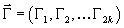
Γ = (Γ₁, Γ₂,…Γ_2k)

be the usual gamma matrices regarded as maps from S_– to S₊. If x = (x₁, x₂,…x_2k) is an element of S^{2k – 1}, meaning a 2k-vector with x² = 1, then we define the tachyon field by

T(x) = Γ . x

It has winding number 1, and generator π_{2k – 1}(U(2^{k – 1})). The p-brane charge is 1, and all higher and lower charges vanish. Since this configuration has p-brane charge 1, and looks like the vacuum except near x = 0, we assume that this is, in fact, a p-brane.

So therefore, a p-brane is equivalent to 2^{k – 1} pairs of (p + 2k)-branes and antibranes. So therefore, a 1-brane is the same as 2^{4 – 1} = 2³ = 8 pairs of (1 + 2(4)) = (1 + 8) = 9-branes and antibranes. A 3-brane is the same as 2^{3 – 1} = 2² = 4 pairs of (3 + 2(3)) = (3 + 6) = 9-branes and antibranes. A 5-brane is the same as 2^{2 – 1} = 2¹ = 2 pairs of (5 + 2(2)) = (5 + 4) = 9-branes and antibranes. A 7-brane is the same as 2^{1 – 1} = 2⁰ = 1 pair of (7 + 2(1)) = (7 + 2) = 9-branes and antibranes. A 9-brane, of course, is already a 9-brane. Since string theory is 10-dimensional, you can’t have an odd-dimensioned p-brane higher than a 9-brane. So any odd-dimensional p-brane is equivalent to a collection of 9-branes and antibranes. Since the charges of any number of pairs of 9-branes and antibranes can be classified by K-theory, therefore the charges of any odd-dimensional p-brane can also be classified by K-theory.

A D-brane wrapped on a submanifold S of spacetime may carry a nonzero Ramond-Ramond (RR) charge. D-branes carry gauge fields, and these fields are natural in K-theory, which has been used to answer some questions about RR charges and fields.

If X is spacetime, and A(X) is the commutative associative algebra of continuous complex-valued functions on X, then the K-theory of X can be defined in terms of representations of A(X). A representation of a ring is called a module. The most obvious example of an A(X)-module is A(X) itself. For f ∈ A(X), regarded as a ring, and g ∈ A(X), regarded as a module, you have f(g) = fg, where on the right hand side, the multiplication occurs in A(X). This obeys the defining condition of a module which is (f₁ f₂)(g) = f₁(f₂(g)).

Let’s say you have a Dp-brane, or a collection of N Dp-branes, wrapped on a submanifold S of X, with any Chan-Paton gauge bundle W on the Dp-brane. Let M(S) be the space of sections of W, meaning the space of one-particle states for a charged scalar coupled to the bundle W. Then M(S) is an A(X)-module. For f ∈ A(X) and g ∈ M(S), we set f(g) = fg. On the right hand side, the multiplication is defined by restricting f, which is a function on X, to S, and then multiplying f and g. Therefore, in Type IIB superstring theory, a collection of D9-branes defines a representation or module E of A(X). A collection of anti-D9-branes defines another module F. Any configuration of D9 and anti-D9-branes determines a pair (E, F). To classify D-brane charge, you have to classify (E, F) pairs modulo physical processes. A important process is brane-antibrane creation and annihilation, the creation or annihilation of a set of D9’s and anti-D9’s, each having the same gauge bundle G. This would be written as

(E, F) → (E ⊕ G, F ⊕ G)

The equivalence classes make up a group called K(X). You could call it K(A(X)) if you want to emphasize the interpretation in terms of A(X)-modules. D-branes in Type IIB carry conserved charges that take values in K(X).

Whenever you look closely at topological properties of RR charges or fields, you see effects that reflect the K-theory structure. For example, there are stable D-brane states, such as the nonsupersymmetric D0-branes of Type I, that would not exist if D-brane charge were classified by conventional cohomology instead of K-theory. Also, it is possible to have a D-brane state that would be stable if D-brane charge were measured by conventional cohomology, but are in fact unstable due to a process that involves nucleation of D9-[D9 bar] pairs in an intermediate state. This occurs in Type II superstring theory in which a D-brane wrapped on a homologically nontrivial cycle in spacetime is in fact unstable. Also, the K-theory interpretation of D-branes is needed to explain a global worldvolume anomaly.

K-theory can be naturally adapted to stringy generalizations. We defined K(X) in terms of representations of the algebra A(X) of functions on spacetime. We could also define K(A) for any noncommutative algebra A in terms of pairs (E, F) of A-modules. Turning on the Neveu-Schwarz B-field, you can make A(X) noncommutative. The associated K(A) was used by Connes, Douglas, and Schwarz in the original paper on noncommutative Yang-Mills theory applied to string theory. It would be great to have a fully stringy version involving a noncommutative algebra constructed using all the modes of the string, not just the zero modes. One possible candidate for the noncommutative algebra is the *-algebra of open string field theory, defined in terms of gluing strings together. If you call this algebra A_st, it seems plausible that D-brane charge is naturally labeled by K(A_st). For a manifold of large volume compared to the string scale, K(A_st) is the same as ordinary K(X) of topological K-theory.

An RR p-form field G_p obeys a Dirac quantization law according to which, for any p-cycle U in spacetime

∫_U G_p/2π ∈ Z

meaning, is an integer. The actual quantization conditions on RR periods are more subtle than the above equation. There are a variety of corrections to the above equation that involve spacetime curvature and gauge fields on the brane, such as self-duality and global anomalies.

For Type IIB superstrings, it turns out that RR fields are classified by K’(X). For our purposes, K’(X) can be defined as the group of components of the group of continuous maps from X to U(N) for any sufficiently large N, where N is the number of D-branes. This means that topological classes of RR fields on X are classified by a map U: X → U(N) for some large N. The relation of G_p to U is G_p ~ Tr(U^-1 dU)^p, ignoring corrections due to spacetime curvature and the self-duality of the RR fields. We don’t know what U actually is. This is analogous to the fact that RR fields are classified by U(N) gauge bundles, for some large N, with connection A and curvature F_A, where G_p ~ Tr F_A^p/2. M-theory involves E₈ gauge bundles with connection. We don’t really know the physical meaning of the U(N) gauge bundles or the E₈ gauge fields.

Using K’(X) to classify RR fields in Type IIB gives you a way to summarize very complicated quantization conditions obeyed by the RR fields. In addition, this framework is useful in describing subtle phase factors that enter into the RR partition function. When it became known that RR charges were classified by K-theory, people at that time should have immediately realized that RR fields were also classified by K-theory, since RR charges produce RR fields, but it tool a couple of years for people to realize this.

Just like K⁰(X), K¹(X) has an analog for any noncommutative algebra A. Given A, you let A_N denote the group of invertible N x N matrices whose matrix elements are elements of A. Then K’(X) is the group of components of A_N for large N. For example, if A = A(X) is the ring of complex-valued continuous functions on X, then A_N is the group of maps of X to GL(N, C). This is contractible to the group of maps of X to U(N), so for large N, the group of components of A_N is the same as K’(X). The existence of a generalization of K’(X) in the long distance limit might be a useful starting point for stringy generalizations.

Up until now, we’ve assumed that N, the number of D-branes, was a sufficiently large but finite integer. What happens if you set N equal to infinity? There are many examples in string theory where we study the N → ∞ limit. Examples include the conjectured link between strings and gauge theory, the old matrix models that are used to give solvable examples of string theory, the matrix model of M-theory, and the correspondence between gravity in an asymptotically AdS spacetime and conformal field theory (AdS/CFT correspondence). In the present case, it is worthwhile to study D-branes with N = ∞, with tachyon condensation to annihilate most of the branes and reduce it to something more manageable. One question is the relation of Type IIA superstrings to K-theory. Another is the inclusion of a nontrivial topological NS three-form H in the K-theory classification of RR charges and fields.

For Type IIB superstrings, we used K⁰(X) to classify RR charges, and K¹(X) to classify RR fields. Therefore, because of T-duality, it should be reversed for Type IIA superstrings. According to T-duality, for Type IIA superstrings, K¹(X) should classify RR charges, and K¹(X) should classify RR fields. By Bott periodicity, K^{i + 2}(X) = Kⁱ(X), so the only K-groups of X are K⁰(X) and K¹(X). In 1999, Petr Horova came up with the best explanation of why K¹(X) classifies RR charges in Type IIA. Let’s say you have a system of N unstable D9-branes in Type IIA. The branes support a U(N) gauge field and a tachyon field T in the adjoint representation of U(N). There is a symmetry T → -T. The effective potential of the tachyon field has the general form

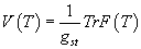
V(T) = (1/g_st) Tr F(T)

where the function F(T) is non-negative, and after scaling T correctly, vanishes precisely if T = ±1. Therefore, V(T) is minimized if and only if every eigenvalue of T = ±1. Horova argued that in flat R¹⁰, you can make supersymmetric Dp-branes, for even p, as solitons of T. For instance, to make a D6-brane, you set N = 2. Let x be the three coordinates normal to the D6-brane, and set

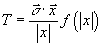
T = ((σ . x)/| x | )f(|x|)

Where f(r) ~ r for small r, and f(r) → ∞ for r → ∞. Then for | x | → ∞, the eigenvalues of T are everywhere ±1. Near x = 0, there is a topological knot that can be interpreted as a D-brane.

In flat R¹⁰, you can make Dp-branes for other even p the same way. You can do it on flat spacetime for any value of N, but you can only do it on curved spacetime if N is equal to infinity. On a general spacetime, this does not work for arbitrary Dp-branes unless you set N = ∞. The problem is most obvious if X, or at least its spatial part, is compact. The tachyon field T, being adjoint-valued, maps X to the Lei algebra of U(N). Since the Lie algebra is contractible, T carries no topology. A map from X to the Lie algebra does not represent an element of K’(X). Since it can be contracted to a point, it carries no topological information.

Therefore, to define an element of K’(X), you need a group, not the Lie algebra. You use the map U : X → U(N). What’s amazing is that if you set N = ∞, you get the correct topology from the Lie algebra. You have to interpret U(∞) to be the unitary group U of a Hilbert space H of countable infinite dimension, which is called a separable Hilbert space. You interpret the N = ∞ analog of the space of hermitian N x N matrices to be the space of bounded self-adjoint operators T on H whose spectrum is as follows. There are infinitely many positive eigenvalues and infinitely many negative eigenvalues. Zero is not an accumulation point on the spectrum which makes T into a Fredholm operator. Physically, T should be required to obey these conditions since they are needed to make the energy and D8-brane charge finite. To make the energy finite, almost all the eigenvalues of T are very close to ±1. With these conditions imposed on T, it turns out that the space of T has the same topology as that of U(N) for large N.

Therefore, you can use tachyon condensation on a system of D9-branes to describe RR charges for Type IIA but you have to start with infinitely many D9-branes which then undergo tachyon condensation down to a configuration of finite energy.

We also want to consider D9-branes when the Neveu-Schwarz three-form H is nontrivial. Just as with H= 0, we want to classify D-brane states by pairs (E, F), when E is a D9-brane, and F is an anti-D9-brane, subject to the usual equivalence relations. However, there is a problem with having a D9-brane in the presence of a Neveu-Schwarz H-field. When H is topologically nontrivial, you can’t have a single D9-brane. On the D9-brane, there is a U(1) gauge field with field strength F. The relation dF = H shows that H must be topologically trivial if a single D9-brane is present. This is most easily shown in de Rham cohomology, but it’s true generally.

Now let’s consider the case where we identify H with torsion, and there is an integer M > 0 such that MH is topologically trivial. Then it is possible to have a set of M D9-branes whose gauge bundle actually has the structure group U(M)/Z_M instead of U(M). The obstruction to lifting the U(M)/Z_M bundle to a U(M) bundle is determined by H. In this case, the gauge bundle is called a twisted bundle. For any positive integer m, you can have N = mM D9-branes with the structure group of the bundle being U(mM)/Z_M. In this case, the D-brane charge is classified by pairs (E, F) of the twisted bundles. The equivalence classes make a group K_H(X).

In order to interpret K_H(X) as the K-theory of representations of an algebra, you have to pick a particular twisted bundle W and consider a D-brane with boundary conditions determined by W. The W-W open strings transform in the adjoint representation, so the gauge parameters of the zero mode sector of the open strings are sections of W ⊗ [W bar]. Notice that although W is a twisted bundle, with structure group U(M)/Z_M rather than U(M), W ⊗ [W bar] is an ordinary bundle, since the center acts trivially in the adjoint representation.

The sections of W ⊗ [W bar] form an algebra. If s_jⁱ and t_l^k are sections of W ⊗ [W bar], where the upper indices are W-valued, and the lower indices are [W bar]-valued, then their product is

(st)_lⁱ = [summation over k]s_kⁱt_l^k

This is the algebra A_W(X) of all endomorphisms or linear transformations of the bundle W. The algebra of open string field theory, for W-W open strings, reduces to A_W if you look only at the zero modes of the strings. This is a good approximation t low energies where X is large compared to the string scale.

If H is zero, and W is a trivial rank one complex bundle, then A_W(X) is just A(X). If H is zero, and W is a trivial rank N complex bundle, then including W means just that there are N x N Chan-Paton matrices everywhere. Therefore, in this case, A_W(X) = A(X) ⊗ M_N where M_N is the algebra of N x N complex-valued matrices. In general, whatever H is, W is always trivial locally, so locally A_W(X) is isomorphic to A(X) ⊗ M_N.

A twisted bundle is equivalent to an A_W-module, and the group K_H(X) of pairs (E, F) of twisted bundles, modulo the usual equivalence, coincides with K(A_W), the K-group of A_W-modules. Therefore, K_H(X), as defined in terms of pairs (E, F) of twisted bundles, is manifestly independent of W, while K(A_W) appears to depend on W. Given any two distinct twisted bundles W and W’, the corresponding algebras A_W and A_W’, are distinct but are Morita equivalent, which implies that K(A_W) = K(A_W’).

So far, we have assumed that H is torsion. A typical example, important in AdS/CFT correspondence, is the spacetime X = AdS₅ x RP⁵, where a torsion H-field on RP⁵ is used to describe Sp(n) rather than SO(2n) gauge theory in the boundary CFT. However, in most cases, H is not torsion. In that case, we must somehow take a large M limit of what we have just done. This was worked out by Bouknegt and Mathai, and independently by Atiyah and Segel. The suitable large M limit of U(M)/Z_M is PU(H) = U(H)/U(1). In other words, for M = ∞, you replace Z_M by U(1). This means that when H is not torsion, you can’t have a finite set of D9-branes and anti-D9-branes, but you can have an infinite set, with a suitable infinite rank twisted gauge bundle E or F. Then the D-brane charge is classified by the group K_H of pairs (E, F) modulo the usual equivalence relations. Kuiper’s theorem, which in involves the contractability of U = U(H), plays an important role. The construction in the M = ∞ limit has the property that the noncommutative algebra whose K-group is K_H is unique, independent of any arbitrary choice of twisted bundles W or W’. This depends on the number of D9-branes and anti-D9-branes being infinite.

Suppose spacetime is a product of cycles [curly W] ⊂ X₉ where X₉ is a 9-dimensional space, possibly noncompact. What are the possible cycles [curly W] ⊂ X₉ which can be wrapped by a D-brane? The answer must meet the following two conditions.

1. The field theory on the D-brane must be consistent. For example, it must be anomaly free. This can put restrictions on the possible cycles on which free D-branes can wrap. Free D-branes are D-branes with no other branes ending on them.

2. We must identify branes which can be dynamically transformed into each other.

In the classification of D-brane charges in Type II string theory, the above conditions are met as follows.

1. A D-brane can wrap [curly W] ⊂ X₉ only if

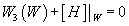
W₃([curly W]) + [H] |_{[curly W]} = 0

In H³([curly W], Z) where W₃([curly W]) is the integral Stiefel-Whitney class of T[curly W]. Specifically, in de Rahm cohomology

[H]_DR|_{[curly W]} = 0

A similar condition applies to other string theories. For instance, in the bosonic string, you have the same condition without the W₃([curly W]) term.

[H] |_{[curly W]} = 0

2. Branes wrapping homologically nontrivial [curly W] can nevertheless be unstable if, for some [curly W]’ ⊂ X₉

PD([curly W] ⊂ [curly W]’) = W₃([curly W]’) + [H] |_{[curly W]’}

Where the left hand side denotes the Poincare dual of [curly W] in [curly W]’. With the bosonic string, the issue of stability is complicated by the fact that the bosonic string includes tachyons, and is thus unstable for that reason. It is not always easy to disentangle the instability associated with the ordinary tachyon, which is always present in the bosonic string, from the instability of the brane, which is what we’re interested in.

First of all, free branes can wrap any homologically nontrivial cycle in X₉. Second of all, a brane wrapping a nontrivial cycle is absolutely stable. Therefore, the homotopy classes of configurations of free branes can be labeled as

H_cpt*(X₉; Z) ~ H*(X₉; Z)

Imposing the above conditions is related to K-theory, and is closely related to a mathematical algorithm for computing K-theory called the Atiyah-Hirzebruch spectral sequence (AHSS), including the AHSS in the presence of non-torsion H-fields. The above two conditions are related to the computation of the AHSS at the third differential. Of course, the AHSS only gives an approximation of K-theory, since it is based on a filtration, and you gave to then solve an extension problem. Our improved understanding of the physical basis of the AHSS clarifies the physical basis for using the mathematical group K_H*(X) for the classification of D-brane charges in the presence of a cohomologically nontrivial H-field. In Witten’s original paper, his argument only applied to the case where [H] was a torsion class. P. Bouwknegt and V. Mathai pointed out that the mathematical theory of K_H*(X) makes perfectly good sense when H is nontorsion, and has a natural formulation in terms of C*-algebras.

The D-branes fall into superselection sectors which are labeled by their charges. The configurations which are referred to as instantons represent transitions between different sectors. Let’s say you have a transition from brane configuration A_i to a brane configuration A_f. It is achieved by an interpolation A(t) with boundary conditions A(t_i) = A_i and A(t_f) = A_f. The interpolation A(t) is an instanton. It is also a D-brane in space X₉.

The discussion depends on the topology of X₉ and the various branes, not on the geometry. If more information on the dynamics is given, then the D-branes A should be stationary in the equations of motion, and A(t) must satisfy the time dependent equations of motion where the parameter t is time. Then an important distinction should be made between two situations regarding the interpolation A(t).

1. When the transition between A_i and A_f is a classically allowed transition, the interpolation A(t) should satisfy the equations of motion with Lorentzian signature.

2. When the transition between A_i and A_f involves tunneling, and is not allowed classically, A(t) should satisfy the equations of motion with Euclidean signature.

Let’s look again at the first condition.

1. A D-brane can wrap [curly W] ⊂ X₉ only if

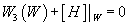
W₃([curly W]) + [H] |_{[curly W]} = 0

In H³([curly W], Z) where W₃([curly W]) is the integral Stiefel-Whitney class of T[curly W]. In the de Rahm theory

[H]_DR |_{[curly W]} = 0

In the de Rahm theory, it simply comes about since the H-field must be trivialized on the D-brane by the equations of motion

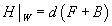
H|_{[curly W]} = d(F + B)

At the level of integral cohomology, the above condition follows from the cancellation of global anomalies for fundamental open strings ending on the D-brane.

Here is the second condition.

2. Branes wrapping homologically nontrivial [curly W] can nevertheless be unstable if, for some [curly W]’ ⊂ X₉

PD([curly W] ⊂ [curly W]’) = W₃([curly W]’) + [H] |_{[curly W]’}

Where the left hand side denotes the Poincare dual of [curly W] in [curly W]’.

To explain the second condition, let’s say you have a cycle [curly W]’ ⊂ X₉ on which

W₃([curly W]’) + [H] |_{[curly W]’} ≠ 0

You can’t wrap a D-brane on [curly W]’, but let’s do it anyway with a D-brane instanton. We can then cancel the global anomalies on the D-brane worldvolume [curly W]’ by adding a magnetic source F on [curly W] ⊂ [curly W]’ such that

PD([curly W] ⊂ [curly W]’) = W₃([curly W]’) + [H] |_{[curly W]’}

A D-brane ending on [curly w] provides just such a magnetic source. Therefore, what you end up with is that a brane wrapping a spatial cycle [curly W] propagates in time, and then terminates on a D-instanton wrapping [curly W]’. This means the brane wrapping the spatial cycle [curly w] can be unstable and decays due to D-brane instantons wrapping [curly W]’.

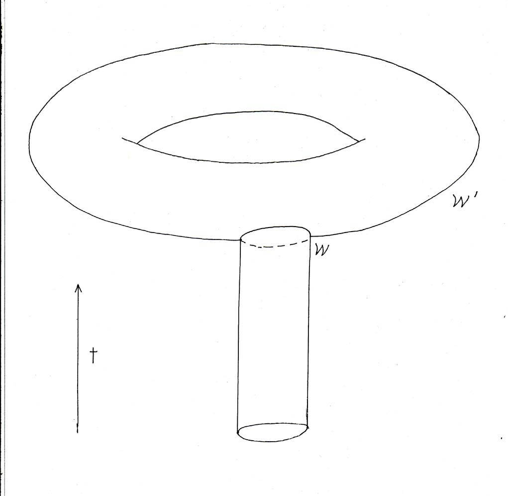
This only means that the brane wrapping [curly W] might decay. The brane wrapping [curly W] could be carrying other conserved charges that prevent decay to the vacuum. This is because we are only addressing the question of which cycles can be wrapped, and not addressing the full question of branes within branes, The second question can be answered by K-theory.

Now let’s show why the second condition does not really cancel the anomalies. In the de Rahm theory, this is easy since by the definition of a magnetic source

dF = 2πPD([curly W] ⊂ [curly W]’)

To extend the argument to the integral condition, you proceed as follows. For simplicity, we’ll put H = 0 but allow W₃([curly W]’) to be nonzero.

Let’s say you have a D-instanton wrapping [curly W]’ where W₃([curly W]’) is nonzero. Then let’s say another D-brane wraps [curly W] x R_t and ends on [curly W]’. In this situation, you can cancel the Freed-Witten anomaly if

PD([curly W] → [curly W]’) = W₃([curly W]’)

Remember that the Freed-Witten anomaly is based on the sign ambiguity in the definition of the path integral for worldsheet fermions. Therefore, you have a family of open string worldsheets S_t, 0 ≤ t ≤ 1, ending on [curly W]’ where S₀ = S₁.

The boundaries of these worldsheets ∂S_t sweep out a 2-cycle

Σ₂ = ∂S ⊂ [curly W]’

where S is the total space of the family. The holonomy of the fermion determinants around S¹ is

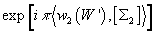
exp[iπ2([curly W]’, [Σ₂]>]

Freed and Witten then extended the condition to require that this factor be unity for any 2-cycle. Σ₂ ⊂ [curly W]’. We will assume for simplicity that the anomaly is due to a 2-cycle Σ₂ with 2Σ₂ = ∂D₃ for some chain D₃ ⊂ [curly W]’. You can learn about Σ₂ by reviewing the definition of the mod-two Bockstein map relating w₂ and W₃. We begin by lifting w₂ to an integral cochain [w bar]₂ such that

<[w]₂, C₂> = <[w bar]₂, C₂> mod 2

for any 2-chain C₂. Now

<[w bar]₂, Σ₂>

is an integer. If 2C₂ = ∂D₃ then

2<[w bar]₂, C₂> = <δ[w bar]₂, D₃> = 23, D₃>

by the definition of the Bockstein, and since this is an equation of integers, you can divide by 2 to get

<[w bar]₂, C₂> = 3, D₃> mod 2

Now let’s apply this to our cycle Σ₂. Note that 3, D₃) is the oriented intersection number of D₃ with PD(W₃). So you see an anomaly will appear when there is a cycle Σ₂ that links the worldvolume [curly W] of the terminating D-brane. In the presence of a magnetic source there is an extra term in the path integral of the form

exp[i ∫_∂St A]

where S_t is the open string worldsheet. The extra factor cancels the ambiguity in the fermion determinant since

∫_∂D3 (F/2π) = 1

so therefore

∫_σ2 (F/2π) = ½

and therefore the magnetic source along [curly W] leads to a factor

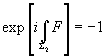
exp[i ∫_Σ2 F] = 1

canceling the ambiguous sign in the fermion determinant.

Let’s say you have DO-brane number in a spacetime with no torsion. The worldvolume of N D)’s defines a 0-cycle W₀ which is Poincare dual to N_X9 where X₉ generates H₉(X; Z) = Z, where X is connected and oriented. We identify N with the 0-brane number in the approximation

H_cpt^odd = k

However, if Σ₃ is any 3-cycle in spacetime on which

∫_Σ3 H = k

then you can consider a D2-instanton wrapping Σ₃. This instanton will violate D0-charge since k worldlines of D0-branes must end on Σ₃. The reason is because these end on monopoles, which are (2 + 1)-dimensional instantons for the U(1) field strengths of the D2-branew so if k worldlines of D0’s end on a D2-brane at positions x_i ∈ Σ₃, then

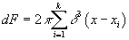
dF = 2π [summation of i from 1 to k] δ³ (x – x_i)

In terms of cohomology, we are identifying

N_X9 ~N_X9 + H ∧ PD(Σ₃)

And since

∫_Σ3 H = k

we know that

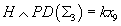
H ∧ PD(Σ₃) = kx₉

So we have the identification N ~N + k. Therefore, D0-brane number is only defined modulo k, and the charge group has at least k-torsion. The same phenomenon shows that other D-instantons induce k-torsion for other charges. For example, a D2-brane wrapping

[summation over i] n_iw_i

where w_i form a basis if H₂(X, Z) has a Poincare dual 7-form ω₇ = n_iω₇ⁱ. D4-instantons wrapping

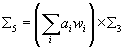
Σ₅ = ([summation over i]a_iw_i) x Σ₃

lead to the identification n_i ~n_i + ka_i. A d4-instanton wrapping a 5-manifld Σ₅ violates the rule [H] = 0. To account for the trivialization dF = dF + H, you must have D2-brane worldvolumes ending on the homology class k(Σ a_iw_i) in Σ₅.

As an example with torsion in H_cpt*(X, Z), let’s say you have a simple example with H = 0. Let’s say c = Sq³(c₀) for some c₀ ∈ H³(X, Z). Then c is Sq³ closed, and thus corresponds to some K-theory class. Therefore, it is also Sq³ exact, and its K-theory lift is zero. Since its K-theory charges vanishes, you would expect a brane with PD(c) = [curly W] to decay. Physically, PD(c) = Q₃ is the homology class of a cycle which is wrapped by a D5-brane instanton. Since Sq³(c₀) is nonzero, Q₆is not spin^c.

You can cancel the global anomalies by allowing the worldvolume Q₃ of the D3-brane to end on Q₆ provided

PD(Q₃ → Q₆) = W₃(Q₆)

Next, I’m going to discuss the Atiyah-Hirzebruch spectral sequence or AHSS. A K-theory class X in K*(X) determines a system of integral cohomology classes. If X ∈ K⁰(X), these are Chern classes c_i(X) ∈ H²ⁱ(X, Z). If X ∈ K¹(X), there are classes ω_{2i + 1} ∈ H^{2i + 1}(X, Z) related to Chern-Simons invariants. However, if you have such a system of cohomology classes, it did not in general come from a K-theory class. The AHSS is a successive approximation scheme for computing the necessary relations on the classes. In each step of the process, you take the results from the last approximation to do the next approximation. In the first approximation

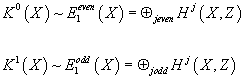
K⁰(X) ~ E₁^even(X) = ⊕_{j even} H^j(X, Z)

K¹(X) ~ E₁^odd(X) = ⊕_{j odd} H^j(X, Z)

Using the differential, d₃ : H^j(X, Z) → H^{j + 3}(X; Z) where (d₃)² = 0, you compute

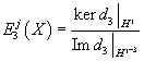
E₃^j(X) = (ker d₃ |_H^j)/ (Im d₃ |_{H^{j + 3}})

and set

E₃^even = ⊕_{j even} E₃^j(X)

to obtain the first correction

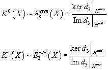
K⁰(X) ~E₃^even(X) = (ker d₃ |_H^even)/(Im d₃ |_H^odd)

K¹(X) ~H₃^odd(X) = (ker d₃ |_H^odd)/(Im d₃ |_H^even)

Then, using the differential d₅ : E₃^j(X, Z) → E₃^{j + 5}(X; Z) you compute

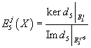
E₅^j(X) = (ker d₅ |_E3^j)/(Im d₅ |_{E3^{j – 5}})

to get the next approximation, and then you just continue the process. You keep computing cohomology in this way to get E_∞^j(X). The procedure is guaranteed to stop after a finite number of steps as long as X is finite dimensional. Then the associated group Gr(X) is defined by

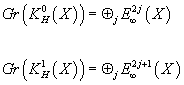
Gr(K_H⁰(X)) = ⊕_j E_∞^2j(X)

GR(K_H¹(X)) = ⊕_j^{2j + 1}(X)

In good cases, you can identify Gr(K) = K. The AHSS is useful because it’s a clearly defined algorithm.

One problem is that you obviously need to have expressions for the differentials, d₃, d₅, etc. The initial term of the spectral sequence is C*(X, h*(pt)), for any generalized cohomology theory h*. A simple expression for the differential d₃ is known. In ordinary K-theory, Atiyah and Hirzebruch identified it as the third Steenrod square, d₃ = Sq³. For twisted K-theory, d₃ = Sq³ + H, in the context of C*-algebra. In de Rahm theory, you get the simple expression

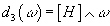
D₃(ω) = [H] ∧ ω

In general, not much is known about the higher differentials. There are scattered results for H = 0, and it appears that nothing is further is known for H nonzero. Fortunately, on compact spin 10-folds at H = 0, you don’t need the higher differentials.

Another problem is that the AHSS is only an approximation to K_H*(X). Let’s say you have a cell decomposition or simplicial decomposition, X₀ ⊂ X₁ ⊂ X₂ …..⊂ X_n. Then we define K_p*(X) to be the classes which become trivial upon restriction to X_p. Obviously, K_{P + 1}* ⊂ K_p*(X). The AHSS really computes the associated graded space, which is

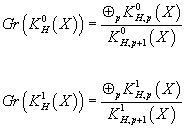
Gr(K_h⁰(X)) = (⊕_p K_{H, p}⁰(X))/(K_{H, p + 1}⁰(X))

Gr(K_H¹(X)) = (⊕_p K_{H, p}¹(X))/(K_{H, P + 1}¹(X))

When you go from that to the full K-theory group, you need to solve an extension problem to get the correct torsion group. Fortunately, in many cases, there is either no extension problem, or it’s not severe. However, there are important examples, such as the compact Lie groups of rank greater than two, and homogeneous spaces, where this complication can be significant. Also, the extension problem is important for orbifolds.

Remember, we are working on spacetimes of the form R x X₉. Let’s say you have a brane wrapping a p-manifold [curly W] ⊂ X₉. You can associate to [curly W] several topological classes. First of all, [curly W] has an associated homology cycle

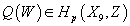
Q([curly W]) ∈ H_p(X₉, Z)

Since X₉ is oriented, there is a Poincare dual integral cohomology class

η([curly W]) ∈ H_cpt^{9 – p}(X₉, Z)

Furthermore, the brane wrapping [curly W] has gauge fields and consequently the D-brane charge is really associated with a class in the K-theory of X₉. The homology class Q can be extracted from the K-theory class, since Q represents the support of the K-theory class.

If the D-brane is realized by tachyon condensation, the support is the locus where the tachyon field vanishes. You then get a cohomology class from η = PD(Q). More generally, to a collection (ω₁, ω₂,…ω₉), we associate a collection of branes by taking Poincare duals to obtain a collection of spatial cycles (PD(ω₁), PD(ω₂),…PD(ω₉)) around which D8, D6,…D0-branes are wrapped. A necessary condition for a cohomology class

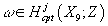
ω ∈ H_cpt^j(X₉; Z)

to survive E_∞^j is that

d₃(ω) = (Sq³ + [H])ω = 0

This is replaced by the anomaly cancellation condition. We therefore interpret d₃(ω) = 0 as a partial requirement for global anomaly cancellation. In fact, it is a weaker condition than

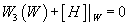
W₃([curly W]) + [H]|_{[curly W]} = 0

It was once believed that in the absence of D-branes, Ramond-Ramond field strengths were classified by twisted K-theory. Evidence for this conjecture came from an analysis of symmetric boundary conditions in the worldvolume theories of open strings, from the analysis of the Chan-Paton bundles on various unstable D-branes, and from the conditions imposed on D-brane embedding by global worldsheet anomaly cancellation. However, within a few years, Diaconescu, Moore, and Witten realized that, in Type IIB superstring theory, the twisted K-theory classification of fluxes is inconsistent with S-duality. This shouldn’t have been surprising since none of the evidence for this conjecture that I listed above is covariant with respect to S-duality. For example, searching for D-branes as boundary conditions in the conformal field theories will not yield an S-duality covariant classification of branes unless you also include Neveu-Schwarz branes, and examine the boundary conditions of (p, q)-strings, which would be difficult as the fundamental string coupling diverges near an NS5-brane. Witten’s construction of untwisted K-theory from tachyon condensation of stacks of D9 and anti-D9-branes also could not be S-dualized as D9-branes are already poorly understood, and their S-duals are unknown if they exist at all. Freed and Witten’s worldsheet anomaly was easily S-duality covariantized. However, except in the case of 3-form field strengths, it was not known how to use it to find a consistency condition for field strengths.

One possible solution to this problem is to use the BRST formalism. You can identify a set of large Ramond-Ramond gauge transformations using the Type II supergravity action, which are essentially those which keep the Wilson loops invariant. These symmetries act on the integral lattice of de Rahm cohomology which satisfies the Dirac quantization condition. This lattice is often smaller than the full integral cohomology, in which the various field strengths are believed to be valued. You use the Freed-Witten anomaly to extend the gauge transformations to the full integral cohomology. The BRST cohomology of the RR gauge transformations is isomorphic, as a set, to twisted K-theory. Atiyah and Hirzebruch showed that K-theory may be constructed from integral cohomology by taking its cohomology with respect to a series of differential operators. In other words, a quotient of a subset of cohomology approximates K-theory, and if you take a quotient of a subset of that, you get a better approximation. Jarah Evslin showed that Atiyah and Hirzebruch’s differential operators are the same as BRST charges corresponding to the large RR gauge transformations. In addition, the extra wrong degree cohomology classes that you add to the sequence are the ghosts and antighosts. This is an unusual application of the BRST formalism because the gauge symmetry is discrete, so the ghosts and antighosts don’t have propagating degrees of freedom. This all suggests that to find the S-duality covariant classification of RR and NSNS field strengths in Type IIB, and also the correct classification in Type IIA, you need to take the BRST cohomology, not only with respect to the RR gauge transformations, but also with respect to the NSNS gauge transformations. However, the NS 3-form field strength is itself used in the RR gauge transformations, and therefore these two symmetries can’t be disentangled. The result is that the collection of NSNS and RR field strengths together don’t form a cohomology or even an additive group. This shouldn’t come as a surprise since the field strengths are solutions to supergravity equations of motion which are nonlinear. When you quotient by the NSNS transformations, you lose more than just the addition. The S-duality covariant classification usually has a different cardinality than the twisted K-theory, as was shown in the case of Klebanov-Strassler geometry.

Edward Witten has speculated that there may be a twisted K-theory based formulation of Type II string theories. However, efforts at constructing such a formulation have been complicated by the fact that twisted K-theory classes are not easily expressed as fields, and so are not easily treated using the standard tools of quantum field theories. However, using the BRST construction, you only need to start with fields that are ordinary differential forms, supplemented with the Dirac quantization conditions, and the various ghost towers that construct a Deligne cohomology and the description of the torsion classes. That is, the field content is the same as the p-form gauge theory. Then you find the symmetries of the path integral, include the ghosts, and calculate the BRST cohomology.

This gives a BRST cohomology which is larger than twisted K-theory. In order to get twisted K-theory you have to ignore the values of the various Wilson lines, which are exponentials of the integrals of the gauge connections. You could also not ignore them, in which such case, you get a differential version of twisted K-theory. The description of the twisted K-theory of spacetime M as a BRST cohomology is summarized as follows, using Type IIA as an example.

BRST	K-theory	Type IIA Supergravity	Type IIA String Theory
fields	⊕kH2k(M)	RR diff. Forms G2k	RR integral classes G2k
ghosts	⊕kH2k + 1(M)	gauge x forms/branes	gauge xforms/branes
BRST operator	d2p + 1	d3 = H∧	=d3 = Sq3 + HU, d5
gauge x forms	d : Hodd → Heven	Wilson loops	FW monodromy
constraints	d : Heven → Hodd	Bianchi identities	source FW anomaly
physical fields	KH0(M)	orbits of Bianchi identities	orbits of FW solutions
anomalies	KH1(M)	stable p-branes	stable D-branes

Stable consistent D-branes correspond to anomalies, despite the fact that their partition functions are gauge invariant. In fact, they appear in the supergravity equations of motion as violations of the conservation of RR current. They also correspond to anomalies as instantonic D-branes which form, sweep out nontrivial cycles, and then decay, changing the cohomology class of fluxes that they source, and therefore mediate a tunneling between different source-free RR solutions.

Notice that on their worldvolumes, the unimproved field strengths are not defined, similar to the worldvolume of a magnetic monopole in QED where the gauge potential A is not defined. In the quantum theory, this may correspond to a nontrivial inner product between states with stable D-branes and states with Ramond-Ramond fields that are pure gauge. The fact that D-branes correspond to elements of the BRST cohomology, and specifically are BRST closed, implies a sort of Wess-Zumino consistency condition, which is enforced classically by the supergravity equations of motion, and quantum mechanically by the Freed-Witten (FW) anomaly.

The field content of eleven-dimensional supergravity is (g, C₃, ψ₁), where g is the metric tensor, C₃ is the antisymmetric tensor field, usually called the C-field, and ψ₁ is the Rarita-Schwinger field, which is a fermion field with spin 3/2. The Lagrangian of the supergravity theory is simple compared to other higher dimensional supergravity theories. It is made of kinetic terms for the three fields involved, and in addition, contains an important piece dictated by supersymmetry, the Chern-Simons term, which is a topological term independent of the metric. If you include quantum effects of anomalies, then you also add a one-loop term made of C₃ and some eight-dimensional polynomial in the Pontryagin class of the tangent bundle of the eleven manifold Y₁₁.

Varying the action of 11d supergravity with respect to each of its fields leads to a set of three equations of motion, which are the Einstein equation for g, the Maxwell-like equation for C₃, and the Rarita-Schwinger equation for ψ. It’s very difficult to solve these differential equations so you only do it in particular cases. Among the interesting solutions are the membrane M2 and the fivebrane M5. These are characterized by being BPS. This means that they are stable against perturbations, and thus do not receive quantum corrections. This implies that such solutions can be trusted in the quantum theory, meaning at strong coupling.

M-theory is a quantum theory in eleven dimensions whose weak coupling limit is classical eleven-dimensional supergravity. There is no intrinsic formulation of the theory without using its limits. There are proposals for such definitions, such as the matrix model, but they have their limitations, especially as far as topology. M-theory also connects the various string theories through a web of dualities, such as perturbative target space T-duality, and nonperturbative strong-weak coupling S-duality. So you can try to study M-theory from its low energy limit which is eleven-dimensional supergravity, or from its connection to the duality web. In the first approach, you use the BPS solutions as objects in M-theory itself.

The degree three field C₃ is responsible for the nontrivial topology of M-theory. In analogy to electromagnetism, where the one-form potential couples to the worldline of the electron, and its dual couples to the worldline of the monopole, you have an analogous situation here where C₃, viewed as an electric potential, couples to the worldvolume of the M2-brane, and the dual potential C₆, viewed as a magnetic potential, couples to the worldvolume of the M5-brane. This is due to the eleven-dimensional Hodge duality between G₄ = dC₃ and *G₄ = dC₆ + … and follows directly from the equations of motion for C₃. In supergravity, the non-gravitational fields are usually taken to be differential forms. However, when you take anomalies into account, such fields are expected to form classes in integral cohomology. However, the situation is usually more subtle. For the case of G₄, you get a shifted quantization condition

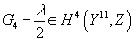
G₄ – (λ/2) ∈ H⁴(Y¹¹, Z)

Where λ is half the Pontryagin class of TY¹¹.

Motivated by the E₈ x E₈ heterotic string theory on the boundary of Y¹¹, Edward Witten showed that G₄ can be interpreted as the class of an E₈ bundle in the eleven dimensions. In 2003, Jarah Evslin and Hisham Sati analyzed the question of supersymmetry in such a theory, and gave an approximate construction of the 11d gravitino as a condensate of the gauge theory fields.

The Kaluza-Klein dimensional reduction of eleven-dimensional supergravity leads to Type IIA supergravity theory whose bosonic field content includes the Ramond-Ramond (RR) fields F_2p (p = 1, 2, …5), and the Neveu-Schwarz (NSNS) field H₃. V. Mathai and Hisham Sati performed the dimensional reduction. In Type II string theories on X¹⁰, you have refinements of the cohomology description, except in this case, you are led to K-theory, K⁰(X¹⁰) for Type IIA, and K¹(X¹⁰) for Type IIB. In the presence of H₃, the corresponding K-theories are twisted. The reduction of E₈ to ten dimensions leads to an LE₈ bundle. This was first proposed by A. Adams and Hisham Sati, where H₃ serves as an obstruction to lifting the loop group bundle to its central extension. This bundle picture can be considered complementary to the twisted K-theory view. Adding a cosmological constant F₀ leads necessarily to an H₃ which is trivial in cohomology, meaning H₃ = dB₂. Instead of looking at the fields, you can look at it from the point of view of D-branes. These are used in homology, and you can go back and forth between cohomology and homology using Poincare duality. There is an analogy with electromagnetism where the branes act as sources of charges that appear as delta-function violations of the corresponding Bianchi identities. This can be viewed as a higher degree analog of Dirac charge quantization for monopoles. The Antiyah-Hirzebruch spectral sequence (AHSS) serves as a tool to detect the difference between cohomology and K-theory, and is thus a powerful tool for D-brane realization. Jarah Evslin proposed a modification of the AHSS in order to describe the group of conserved RR and NSNS charges.

The correspondence between M-theory and Type IIA string theory holds at the quantum level in the path integral formulation, meaning at the level of partition functions. The former is governed by E₈ gauge theory, and the latter by K-theory. The corresponding match for twisted K-theory was started by V. Mathai and H. Sati, where a nontrivial M-theory circle bundle is considered, the NSNS field H₃ nontrivial in cohomology is added, and the corresponding vector bundles are taken not to be lifted from the base. The construction of the K-theory torus is done as in the untwisted case. You also see the appearance of eta differential forms, which are higher degree generalizations of the eta invariant.

The partition function in Diaconescu, Moore, and Witten’s theory has an anomaly given by the seventh integral Stiefel-Whitney class W₇. In 2004, Igor Kriz and Hisham Sati showed that the vanishing of this anomaly is equivalent to orientability of spacetime with respect to complex elliptic cohomology E. Motivated by this, an ellitpic cohomology correction to the Type IIA partition function was defined. The generators of E were proposed as corresponding to M2 and M5-branes in the M-theory limit. Other aspects of string theory also point to elliptic cohomology. In the presence of background NSNS flux, the description of the RR fields in Type IIB string theory using twisted K-theory is not compatible with S-duality. In 2005, Igor Kriz and Hisham Sati showed that other possible variants of twisted K-theory would still not resolve this issue, and proposed a possible resolution using elliptic cohomology. Another piece of evidence for elliptic cohomology is modularity in Type IIB, where there is an elliptic curve that lifts the theory to twelve-dimensional F-theory. Kriz and Sati interpreted this elliptic curve in terms of elliptic cohomology.

The above elliptic cohomology description in Type II string theory can, at least mathematically, be continued to M-theory via a Kunneth formula for E. You can then ask whether E will ultimately be the theory describing the fields of M-theory. Related to this is trying to understand the nature of G₄. For this purpose, in 2005, Hisham Sati wrote the Chern-Simons terms and the one-loop terms n the M-theory action in terms of new characters involving the M-theory four-form and the string classes. The latter are defined as analogs to the usual string class of rank four, λ_i = p_i/2. This suggests the existence of a theory of higher characteristic classes, where the Chern classes and Chern characters are replaced by those new classes and characters. This formalism can be used to give a unified expression for the class of G₄ and its dual, called the Θ class, in analogy with the K-theoretic quantization of the RR fields.

Diaconecsu, Moore, and Witten have shown that the topological part of the M-theory partition function is an invariant of an E₈ gauge bundle over the 11-dimensional bulk. Normally, an 11d gauge theory can’t exhibit linearly realized supersymmetry, but here the gauge theory is nonsupersymmetric and flows to 11d supergravity only in the infrared, with supersymmetry arising as a low energy accidental degeneracy.

In 1996, Horova and Witten demonstrated that when M-theory is compactified on a manifold with boundary, the anomalies caused by chiral gauginos and gravitinos on each boundary component precisely cancel the anomalies that flow in from the bulk. This cancellation occurs only if each boundary component supports precisely 248 10-dimensional vector multiplets,. All transforming in the adjoint representation of E₈. Furthermore, the topological contribution to the M-theory partition function is in fact an invariant of the Dirac operator of a mysterious 11-dimensional E₈ gauge theory. While the nature of the gage theory is unknown, the anomaly cancellation of Horova and Witten, as well as the 10-dimensional N = 1 supersymmetry on every boundary component, place strong constraints on its construction. For simplicity, we restrict ourselves to the case of flat, topologically nontrivial 11-dimensional space, and also neglect higher order Fermi field contributions.

E₈ gauge invariance combined with local supersymmetry invariance requires the relation

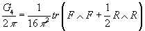
G₄/2π = (1/16π²) tr (F ∧ F + (1/2)R ∧ R)

Between the 11d 4-form field strength G₄ and the 10D N = 1 supersymmetry vector multiplets field strength F on every 10-dimensioanl boundary component. Let’s say you have an E₈ gauge bundle such that the above equation holds everywhere in the 11-dimensional bulk. The fact that such a bundle exists is a consequence of M-theory’s shifted flux quantization condition. The uniqueness of this bundle results from the uniquely simple low dimensional topology of the E₈ group manifold.

In addition to the 248 gauge bosons, you also need 248 Majorana gauginos propagating in the 11d bulk, as well as the 11d graviton. Using the above equation, you can construct the 11d supergravity 4-form G₄ from the vectors. Ten dimensional N = 1 supersymmetry covariance allows you to find the analogous construction of a chiral half of the 11-dimensional gravitino. Eleven-dimensional Lorentz invariance allows you to construct the other half. Therefore, each gauge theory configuration is identified with a single supergravity configuration, meaning that the construction can’t be covariant under 11d supersymmetry since the gauge fields are not part of any representation of 11d supersymmetry.

Therefore, you should identify each gauge field configuration with not only the single supergravity configuration given earlier, but with all of the supergravity configurations which are related to that configuration by an 11d supersymmetry transformation. Therefore, supergravity field configurations related by supersymmetry transformations will be identified with the same gauge field configuration, and thus the same physical state. Physically equivalent configurations on the gauge theory side are also equivalent on the supergravity side, and the E₈ gauge transformations are realized as abelian gauge transformations of the M-theory 3-form.

The low energy effective description of M-theory is 11-dimensional supergravity. The fields of this theory live in a single supermultiplet which contains the gravition, the gravitino ψ, and a three-form C₃, whose exterior derivative, times 6, is the four-form field strength G₄. If the dynamics of M-theory are to be formulated in terms of an E₈ gauge theory, it would be great to have relations between the fields of the 11d supermultiplet, and the fields of the gauge theory, which are the 1-form connection A with field strength F, and an adjoint Majorana gaugino χ. Horova and Witten showed that gauge and gravitational anomaly cancellation on any 10-dimensional boundary of M-theory enforces the relation

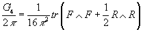
G₄/2π = (1/16π²) tr (F ∧ F + (1/2)R ∧ R)

On the boundary, where R is the curvature 2-form of the tangent bundle.

Witten used locality to argue that such relations, at the level of cohomology, can be extended to the bulk, although it does not follow from this argument that there is an E₈ gauge field strength in the bulk. One reason why there is an E₈ gauge field strength in the bulk is that the low energy effective action for M-theory on the 11-fold Y¹¹ contains the topological terms

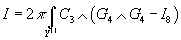
I = 2π [integral over Y¹¹] C₃ ∧ (G₄ ∧ G₄ – I₈)

Where I₈ is a quartic in the curvature tensor. This can be related to a sum of indices of an E₈ gauge theory on an auxiliary 12-dimensional manifold. The ambiguity in I is the integral of its exterior derivative over a closed 12-manifold. The integral may be nonvanishing because C₃ is not necessarily globally defined. The path integral is well-defined if this integral, added to a contribution from the square root of the determinant of the Rarita-Schwinger operator is an integer.

Diaconescu, Moore, and Witten used a theorem of Atiyah, Patodi, and Singer to evaluate the contribution of this topological term and the Pfaffian determinant of the Rarita-Schwinger operator to the phase of the path integral measure.

Φ = Pf(D_RS) e^i∫I = | Pf(D_RS)| exp ((2πi/4) (h_E8 + η_E8) + (2πi/8) (h_RS + η_RS))

where η is the η-invariant of the corresponding operator, which is either the E₈ gauge theory Dirac operator or the Rarita-Schwinger operator, and h is its number of zero modes. So therefore, h_E8 would be the number of zero modes of the E₈ gauge theory operator, η_RS would be the invariant of the Rarita-Schwinger operator, etc. Therefore, a part of the path integral measure of 11-dimensional supergravity can be expressed in terms of the bulk E₈ gauge theory. Also, the partition function consists of a sum over E₈ gauge theory configurations.

At the beginning of my paper “Beyond the Standard Model”, I discuss the different Lie groups, which are defined as the groups of rotations within different types of space. For instance, SO(n) is often described as the group of rotations within real space, although actually it’s the group of rotations within projective real space.

1. So(n) is the group of rotations within real projective space RPⁿ.

2. SU(n) is the group of rotations within complex projective space CPⁿ.

3. Sp(n) is the group of rotations within quaternionic projective space HPⁿ.

4. E₆ is the group of rotations within the projective plane over the bioctonions, (C ⊗ O)P².

5. E₇ is the group of rotations within the projective plane over the quateroctonions (H ⊗ O)P².

6. E₈ is the group of rotations within the projective plane over the octooctonions, (O ⊗ O)P².

7. F₄ is the group of rotations within the projective plane over the octonions, OP².

8. G₂ is the automorphism group of the octonions.

With 248 dimensions, E₈ is the biggest of the exceptional Lie groups, and also the least understood. The easiest way to understand a group is to realize it as the symmetries of a structure you already understand. Of all the simple Lie groups, E₈ is the only one whose smallest nontrivial representation is the adjoint representation. This means that in the context of linear algebra, E₈, is most simply described as the group of symmetries of its own Lie algebra, which is circular reasoning. You can also describe E₈ as the isometry group of a 128-dimensional Riemannian manifold called (O &0times; O)P². However, this manifold is usually defined in terms of E₈ so we’re again stuck with circular reasoning. Nobody knows how to rigorously define (O ⊗ O)P² without first defining E₈. Therefore, E₈ remains enigmatic.

Fortunately, it became slightly less enigmatic recently. Even though the E₈ exceptional Lie algebra was discovered by Wilhelm Killing in 1887, and it was constructed by Eli Cartan in 1894, it was not until 2007 that a team of 18 mathematicians, led by Jeffrey Adams, after four years of hard work and 77 hours on a supercomputer, finally calculated all the representations of E₈. The coefficients of the character formulas for infinite dimensional irreducible representations of E₈ depend on some large square matrices consisting of polynomials called the Lusztig–Vogan polynomials. It was these matrices that the group calculated. The calculation was 60 gigabytes. If you were to try to actually write down the solution, you would need a piece of paper larger than New York City!

Starting from e₈, you can define E₈ to be the simply-connected Lie group with this Lie algebra. The subgroup of E₈ generated by the Lie subalgebra so(16) ⊂ e₈ is Spin(16)/Z₂. This let’s us define the octooctonic plane by

(O ⊗ O)P² = E₈/(Spin(16)/Z₂)

The tangent space at any point of this manifold is isomorphic to S₁₆⁺ ~ (O ⊗ O)P². This partially justifies calling it “octooctonic projective plane”, although it does not satisfy the usual axioms for a projective plane. You can put an E₈-invariant Riemannian metric on the octooctonic projective plane by the technique of averaging over the group action. It turns out that

E₈ ~Isom((O ⊗ O)P²)

So here you have a group defined as the isometry group of a given manifold. However, every group is itself associated with a different manifold which has the holonomy of that group. Therefore, the E₈ group is associated with a manifold called the group manifold E₈. So you have a manifold which is used to define a group which is used to define a different manifold. I’ll give another example of the same thing. Here are some of the holonomy groups of RP³ are

π₁(RP³) = Z₂

π₂(RP³) = 0

π₃ (RP³) = Z

π₄(RP³) = Z₂

The isometry group of RP³ is SO(3), which is associated with the SO(3) manifold. Some of its homotopy groups are

π₁(SO(3)) = Z₂

π₂(SO(3)) = 0

π₃(SO(3)) = Z

π₃(SO(3)) = Z₂

So you have a manifold, say RP³, associated with groups in one way, which are the homotopy groups, say π₁(RP³), and associated with a different group in another way, which is the group of rotations, SO(3), and that group is then associated with its own homotopy groups, such as π₁(SO(3)).

The low dimensional topology of E₈ is in one way, the simplest among nonabelian Lie groups. E₈ has only one nontrivial homotopy group of dimension less than 16, which is π₃(E₈) = Z. This means that on a manifold of dimension less than 16, E₈ bundles are topologically characterized by a single characteristic class, which is the first Pontryagin class.

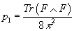
p₁ = (Tr(F ∧ F))/8π²

The only restriction on this class is that its integral over any 4-cycle be an even integer. All other semisimple Lie groups have additional nontrivial low dimensional homotopy groups, and therefore their principle bundles can not be characterized by a single characteristic class. This agrees with what we know about M-theory which at low energies is also described by a 4-form. The 4-form flux of M-theory is a combination of this characteristic class and the first Pontryagin class of the tangent bundle.

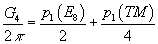
G₄/2π = p₁(E₈)/2 + p₁(TM)/4

Notice that the shifted flux quantization condition of G₄ is automatic in this construction. The first term on the right hand side is an integral cohomology class, while the second term could be an integral cohomology class or could be half an integral cohomology class. Therefore, the failure of the left hand side to be integral is precisely equal to the failure of the second term of the right hand side, or the mod 2 part of p₁(TM)/2.

As a result of the fact than an E₈ bundle is described by a single closed form, an E₈ bundle on a manifold of dimension less than 16, has only one type of topological defect, which is the M5-brane. Of course, if it has M5-branes, then it automatically also has M2-branes. For instance, an M2-brane is created when two M5-branes cross via the Hanany-Witten mechanism. The M5-brane is a codimension 5 defect where the form fails to be closed.

Before I describe the E₈ gauge theory model of M-theory, let’s first describe a simpler case of the ‘t Hooft-Polykov monopole, in order to gain insight into the role of the M5-brane defect. Let’s say you have an SU(2) gauge theory in at least three dimensions with a scalar Φ^a that transforms in the adjoint of SU(2), and is

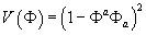
V(Φ) = (1 – Φ^aΦ_a)²

The group SU(2), like E₈, is a simple Lie group, and so π₃(SU(2)) = Z. Therefore, the gauge bundle admits a codimension 5 defect constructed same as the M5-brane is constructed. However, because a configuration of Φ is a map from spacetime to SU(2), the presence of an adjoint Higgs field in this model allows a defect of codimension 3. If you impose a finite energy condition on 3-dimensional slices of spacetime, then on each of these slices, Φ is a map from S³ times an irrelevant space to SU(2) ~ S³. Such a map is classified up to homotopy by an element n ∈ π₃(SU(2)) = Z, where n is the ‘t Hooft-Polykov magnetic monopole charge of the 3-dimesional slice.

The field strength F of a U(1) gauge theory can be constructed from the field strength G^a of the original SU(2) and the scalar field via

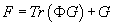
F = Tr (ΦG) + G

In the U(1) gauge theory description, the ‘t Hooft-Polykov monopole appears to be a Dirac monopole in the following sense

[integral over S²] F = 1

for any 2-sphere that links the monopole once. However, at microscopic distances, this abelian effective description breaks down, and the physics, like asymptotic freedom, can’t be understood without the nonabelian description.

This construction could be repeated with an E₈ gauge theory that had a scalar Higgs transforming in the adjoint of E₈. In this case, the configuration of the Higgs field in a 3-plane transverse to the monopole, after a 1-point compactification of this 3-plane, will again be an element n ∈ π₃(E₈) = Z, where n is the monopole charge.

The existence of the adjoint scalar was crucial to the construction of the ‘t Hooft-Polykov monopole. Such a scalar does not exist in the E₈ gauge theory model of M-theory, so you don’t have a ‘t Hooft-Polykov monopole or an abelian two-form field strength. In trying to construct an E₈ scalar from the E₈ field strength, notice that although there is no adjoint scalar with which to contract its E₈ indices, there is the E₈ field strength itself. Specifically, you can construct an abelian four-form [G tilde]₄ from the E₈ field strength via

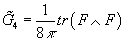
[G tilde]₄ = (1/8π) tr(F ∧ F)

so that F plays the same role as the Higgs field in the example of the monopole. As in the case of the ‘t Hooft-Polykov monopole, this description breaks down at the topological defect, where the nontriviality of π₃(E₈), and thus the nonabelian nature of the original high energy theory becomes impossible to ignore.

Type II string theories in ten dimensions contain, in addition to gravity and fermions, p-form fields, which are the Ramond-Ramond (RR) and Neveu-Schwarz (NS) fields. D-branes are charged under these p-forms. It is by now well known that RR charges in the absence of NS fields can be classified by K-theory of spacetime, specifically K⁰(x) for Type IIB, and K¹(x) for Type IIA. The RR fields are also classified by K-theory with the roles of K⁰(X) and K¹(X) reversed. In the presence of a NS B-field, or its field strength H₃, the fields and the charges are classified by twisted K-theory. It was shown by Freed and Witten by analysis of worldsheet anomalies for the NS field, [H₃] ∈ H³(X, Z) is a torsion class. M-theory is a theory in eleven dimensions which is not yet known except in specific regions or points in its moduli space. Witten showed that the topological part can be encoded in the index theory of an E₈ gauge bundle. At the level of supergravity, the low energy limit of string theories and M-theory, there is an explicit relation between the two given by the Kaluza-Klein relation. Actually, it’s much more subtle at the quantum level due to the existence of nontrivial phase factors in the partition function. E. Diaconescu, G. Moore, and E. Witten showed that you can also relate the corresponding partition functions, specifically the one derived using E₈ gauge theory in eleven dimensions, and the one derived from K-theory in ten dimensions. They restricted themselves mostly to the RR sector. This has been generalized to include the fermions, one-loop contributions, and membrane instantons, as well as including flat background NS potentials. The partition functions are T-duality invariant only after including these effects.

Let’s say Y is an eleven-dimensional spin manifold corresponding to M-theory, and X is a ten-dimensional manifold which is the base space of a circle bundle with total space Y, and corresponds to Type IIA string theory. Z is a twelve-dimensional manifold which is a disk bundle over X, whose boundary is a circle bundle Y over X. The basic set up for the bundles is

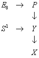
where P is a principle E₈ bundle over the 11-dimensional manifold Y, which is in turn is a principle S¹ bundle over the 10-dimensional manifold X. Then Y has a supergravity field whose field strength is a closed 4-form G₄, that is related to the integral characteristic class invariant a of P by

G₄/2π = a – λ/2

Where λ/2 is equal to half the first Pontryagin class p₁(Y) of Y.

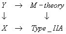
We are interested in the comparison using the metric

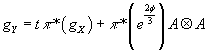
g_Y = tπ*(g_X) + π*(e^2φ/3)A ⊗ A

in the large volume limit as t → ∞.

M-theory has three kinds of impurities which are membranes, five-branes, and boundaries. The low energy theory is eleven-dimensional supergravity. The massless degrees of freedom are the metric g, a three-form potential C₃, and a Rarita-Schwinger fermionic spin 3/2 field ψ_M. The action of eleven-dimensional supergravity is

I₁₁ = I_grav + I_G4 + I_{C. S.} + I_fermi + I_coupling

where

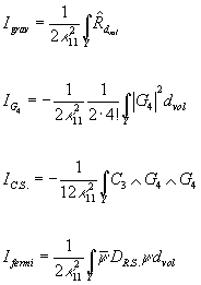
I_grav = 1/ 2κ₁₁² ∫_Y [R hat]d_vol

I_G4 = -1/ 2κ₁₁² (1/2 . 41)∫_Y |G₄|² d_vol

I_{C. S.} = 1/1 2κ₁₁² ∫_Y C₃ ∧ G₄ ∧ G₄

I_fermi = 1/ 2κ₁₁² Â½ ∫_Y [ψ bar] D_{R. S.} &psu;d_vol

where

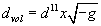
d_vol = d¹¹ x[squareroot of –g]

[R hat] is the scalar curvature of Y, G₄ is the four-form field strength which, when cohomologically trivial, is equal to dC₃. The fermions involve the kinetic action of &psi_M involving the Rarita-Schwinger operator D_{R. S.}. You can view D_{R. S.} as the Dirac operator coupled to the vector bundle associated to the virtual bundle

TY – 3[curly O]

where the [curly O] factors correspond to subtraction of ghosts. I_coupling corresponds to the coupling of &psi_M to G₄, as well as quartic &psi_M self-couplings.

The source-free Bianchi identity and equation of motion are

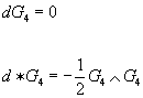
dG₄ = 0

d * G₄ = -½G₄ ∧ G₄

which can be modified by adding sources, such as the M2-brane and M5-brane. They have worldvolumes [curly W]₃ and [curly W]₆ respectively, by an embedding in spacetime Y. There are also one-loop corrections that, for example, modify the right hand side of the above equation by the topological quantity

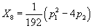
X₈ = (1/192)(p₁² – 4p₂))

given in terms of the Pontryagin classes of the tangent bundle TY. The four-form of M-theory obeys the quantization condition

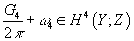
(G₄/2π) + ω₄ ∈ H⁴(Y; Z)

where ω₄ is the fourth Stiefel-Whitney class of the tangent bundle TY. In the orientable case

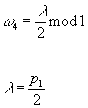
ω₄ = λ/2 mod 1

λ = p₁/2

The M-theory partition function is a product of factors that correspond to different parts of the action.

Z_M ~ Z_gravZ_G4 Z_{C. S.} Z_fermi Z_coupling

We are interested in the topological part of the partition function, which means that we keep only the moduli associated with C₃ or G₄ but keep all the phases so that the part we are interested in is

e^{-|| G₄(a) ||2 Ω_M(C₃)}

Therefore, we do not consider Z_grav or Z_coupling. This theory can be viewed as having two kinds of fermions. First you have the spin ½ fermions in the E₈ gauge theory, and then you have the spin 3/2 Rarita-Schwinger fields in the supergravity. At the level of the action, you have

I_M = I_E8 + I_{R. S.}/2

The low energy quantum measure of M-theory factorizes in terms of manifestly well-defined factors

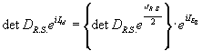
det D_{R. S.} e^iI_M = {det D_{R. S.} e^{iI_{R. S.}/2}} . e^iI_E8

For the second factor, J = e^iE₈. If ∂Y ≠ 0, then J is not gauge-invariant, but is a section of a line bundle L^-1 over the space of C-fields over N = ∂Y.

The expression G₄ = dC₃ is not valid globally, and C₃ is not a well-defined differential form, implying that you have to be careful in defining the topological part I_{C. S.} of the action I₁₁. The way around this is to lift to twelve dimensions, and look at the action.

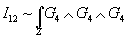
I₁₂ ~ ∫_Z G₄ ∧ G₄ ∧ G₄

over a twelve dimensional manifold Z. The full Chern-Simons coupling of M-theory is associated with I₁₂, which is well-defined and independent of the choice of Z and the extension of G₄. The action can be written as

I₁₂ = -(1/6)a³

where a is the cohomology class of [G₄/2π]. Witten showed that there are two modifications to this. First of all,

a – λ/2

is an integral, and second of all, we have to include

C₃ ∧ X₈

Introduce an E₈ bundle V on Z whose characteristic class ω obeys

ω = a – λ/2

Witten showed that

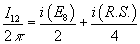
I₁₂/2π = i(E₈)/2 + i(R. S.)/4

and, including the above effects, the action takes the form

I₁₂/2π = -1/6(ω – λ/2)[(ω – λ/2)² – 1/8(p₂ – λ²)]

which is just I_{C. S.} with the gravitational corrections included. For the Rarita-Schwinger path integral, (1/2π)I₁₂ can be half integral in general, and has an anomaly that is cancelled from the one coming from the determinant of the Rarita-Schwinger operator det D_{R. S.}. The combination shows up as

det D_{R. S.} e^{iI_{R. S.}/2}

The Rarita-Schwinger operator can be viewed as the Dirac operator coupled to TX – 2[curly O], since Y is a circle bundle over X, or equivalently to TZ – 4[curly O] in twelve dimensions. Overall, you have the factor

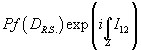
Pf(D_{R. S.}) exp(i∫_Z I₁₂)

where Pf(D_{R. S.}) is a vector in a Pfaffian line, so the above can be factorized into a modulus | Pf(D_{R. S.}) | and a phase

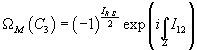
Ω_M(C₃) = (-1)^{I_{R. S.}/2} exp (i ∫_Z I₁₂)

Using the Atiyah-Patodi-Singer (APS) index theorem, you can relate the action to an index corrected by the reduced eta invariant

[η bar] = (h + η)/2

as

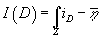
I(D) = ∫_Z i_D – [η bar]

so that the relevant integral in twelve dimensions can be written as

∫_Z I₁₂/2π = ½ I_E8 + ¼ I_{R. S.} + (h_E8 + η_E8)/4 + (h_{R. S.} + η_{R. S.})/8

Now the factor (-1)^{I_{R. S.}} cancels the one coming from the index theorem, and taking into account the fact that the index is even, the phase is

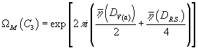
Ω_M(C₃) = exp[2πi ([η bar](D_V(a))/2 + [eta; bar](D_{R. S.})/4)]

The Riemannian metric on the circle bundle Y is

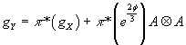
g_Y = π*(g_X) + π*(e^2φ/4)A ⊗ A

where g_X is the Riemannian metric on X, e^2φ/3 is the norm of the Killing vector along S¹, which in this trivialization is given by ∂z, φ is the dilaton, which is a real function on X, and A is a connection 1-form on the circle bundle Y. The component of the curvature in the direction of the circle action is

R₁₁ = e^2φ/3 = g_s^2/3

This choice of Riemannian metric is compatible with the principle bundle structure in the sense that the given circle bundle action acts on the isometries of Y. Performing a rescaling to the above metric, the desired metric ansantz for Type IIA is

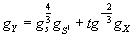
g_Y = g_s^4/3 g_S¹ + tg^-2/3 g_X

in the limit t → ∞, then g_s → 0.

The reduction of the 4-form G₄ on Y gives rise to two differential forms on X, the Neveu-Schwarz 3-form H₃, and the Ramond-Ramond 4-form F₄. This is obtained as follows, setting the dilaton to a constant for simplicity.

For an oriented S¹ bundle with first Chern class

c₁(Y) = F₂ = dA ∈ H²(X, Z)

you have a long exact sequence in cohomology called the Gysin sequence

… → H^k(X, Z) →^π* H^k(Y, Z) →^π* H^{k – 1}(X, Z) →^F∪ H^{k + 1}(X, Z) → …

If k = 4, you see that

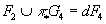
F₂ ∪ π_* G₄ = dF₄

where F₄ is some differential form on X. It follows that

d(A ∧ π_* G₄ + F₄) = 0

Therefore, setting H₃ = π_* G₄, we see that H₃ is a closed form. Noting that π_*(A) = 1, we get the equation on Y, where it is understood that forms on X are pulled back to Y via π.

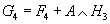
G4 = F₄ + A ∧ H₃

The curvature 2-form F₂ = dA is basic. It is horizontal, i_vF₂ = 0, and invariant, L_vF₂ = 0, where v is a vertical vector. In a local trivialization of the circle bundle where A = dz + θ, where θ is the connection on X, the above two conditions mean that F₂ has no dz component, and that it does not depend explicitly on z. Similarly, G₄ can be written in the given trivialization as

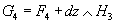
G₄ = F₄ + dz ∧ H₃

Let’s say that G₄ ∈ Ω⁴(Y) and the curvature F₂ ∈ Ω²(X) satisfy the Bianchi identities on Y that are given below, and which are obtained from the Euler-Lagrange equations for the bosonic part of the action of eleven-dimensional supergravity, I_grav + I_G4.

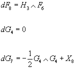
dF₈ = H₃ ∧ F₆

dG₄ = 0

dG₇ = -½G₄ ∧ G₄ + X₈

where F₈ = _*10F₂, F₆ = _*10F₄, G₇ = _*11G₄, and X₈ is a basic differential form of degree 8 on Y, which is a Chern-Simons correction factor. By applying the de Rham differential on the last of the above equations, you can see that X₈ is a closed form. The one-loop coupling ∫ C₃ ∧ X₈ reduces to ∫ B₂ ∧ X₈. When X₈ = 0, and G₄ is proportional to a volume form of a four-dimensional factor in Y, this is the Freund-Rubin ansatz. When G₄ is a flux through four-cycles in Y, there are solutions with X₈ ≠ 0 for different choices of Y. The Bianchi identity dG₄ = 0 reduces to the Bianchi identities for the RR 4-form, NS 3-form, and the RR 2-form field strengths.

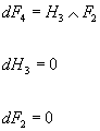
dF₄ = H₃ ∧ F₂

dH₃ = 0

dF₂ = 0

From general principles, you can write G₇ = H₇ + A ∧ F₆ where H₇ and F₆ are basic forms on Y. This is consistent with

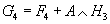
G₄ = F₄ + A ∧ H₃

since you can show that

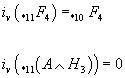
i_v(_*11F₄) = _*10F₄

i_v(_*11(A ∧ H₃)) = 0

You can use

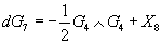
dG₇ = -½G₄ ∧ G₄ + X₈

to show that

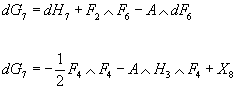
dG₇ = dH₇ + F₂ ∧ F₆ – A ∧ dF₆

dG₇ = -½F₄ ∧ F₄ – A ∧ H₃ ∧ F₄ + X₈

Eliminating dG₇ from the above equations, you get

dH₇ = -F₂ ∧ F₆ + A ∧ (dF₆ – H₃ &and F₄) – ½F₄ ∧ F₄ + X₈

All the terms in the above equation, except for the term involving A, are differential forms. Therefore, contracting the terms of the above equation with the vertical vector field v and using the fact that i_v(A) = 1 and

i_v(dF₆ – H₃ ∧ F₄) = 0

we deduce the corresponding ten-dimensional Bianchi identities on X

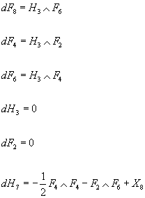
dF₈ = H₃ ∧ F₆

dF₄ = H₃ ∧ F₂

dF₆ = H₃ ∧ F₄

dH₃ = 0

dF₂ = 0

dH₇ = -½F₄ ∧ F₄ – F₂ ∧ F₆ + X₈

From G₄ ∈ Ω⁴(Y) satisfying the eleven-dimensional Bianchi identities, we obtain F = F₂ + F₄ + F₆ + F₈ ∈ Ω^even(X) satisfying (d – H₃ ∧) F = 0, where we observe that F₀ = 0 since H₃ is not exact, and F₈ ∧ H₃ = 0 for dimensional reasons. Therefore, F determines a class in the twisted cohomology H^even(X, H₃) where

H^[dot](X, H₃)

is the twisted cohomology, which is by definition, the cohomology of the Z₂-graded complex

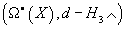
(Ω^[dot](X), d – H₃ ∧)

where the de Rham differential is replaced by

d – H₃ ∧

We are dealing with Dirac operators coupling to certain vector bundles. We are interested in the general case where the vector bundles are not lifted from the base. First of all, you have the twisting by the tangent bundle which leads to the Rarita-Schwinger operator. In this case, you are dealing with natural bundles which are not lifted from the base. Second of all, you also have the Dirac operator coupled to an E₈ vector bundle. In this case, you want to consider it as not lifted from X. Therefore, you have eta-forms in the adiabatic limit of the reduced eta invariant of that Dirac operator.

First we’ll look at the Rarita-Schwinger operator D_{R. S.}. There are two contributions, one from h, and one from η. In 8n + 2 dimensions

h_{D ⊗ VR}

is a topological invariant mod 2. For the contribution from h, the idea is to try to relate the spectrum on Y to that of X.

E. Diaconescu, G. Moore, and E. Witten chose functions Φ that transform as

Φ → e^-ikθ Φ

under an S¹-rotation by an angle θ. The choice of functions depends on whether Y is compact or not. In the compact case, you can choose the functions to be smooth L²(Y) with respect to the metric that respects the circle bundle. In the case, X and Y are not compact, you can decompose the eta function as a sum over contributions from a given k. For k = 0, the phase is the same as the trivial circle bundle

i^{h_{R. S.}+}

where + refers to positive chirality, and for k ≠ 0, there is no contribution from h. The contribution from η, derived by Diaconescu, Moore, and Witten is

η(s)/2 = | R |^s [summation over k from 1 to ∞] (ak^{-(s – 1)} + bk^{-(s – 3)} + ck^{-(s – 5)})

where the coefficients a, b, and c are given in terms of characteristic classes.

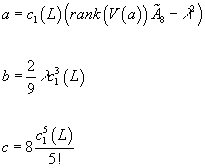
a = c₁(L)(rank (V(a)) [A tilde]₈ – λ²)

b = (2/9) λ c₁³(L)

c = 8c₁⁵(L)/5!

Then the above contributions combine in [η bar]_{R. S.}.

Now let’s look at the E₈-coupled Dirac operator D on Y. We’ll use the method of J. Bismut, J. Cheeger, and X. Dai for calculating the adiabatic limit of the reduced eta invariant. Let’s say R^X is the curvature of X, and SX is its spin connection ∇^X induced from the Levi-Civita connection on X. Associated to the principle E₈ bundle P on X, you have a Hermitian vector bundle V(a) with a unitary connection ∇^V(a). Then the bundle SX ⊗ V(a) has a tensor product connection

∇ = ∇^X ⊗ 1 + 1 ⊗ ∇^V(a)

A natural representation of C1(X_p) on SX_p can be extended to a representation on SX ⊗ V(a). Corresponding to the scaled metric tg^X, you have the Dirac operator D_V(a)⁺, whose reduced eta invariant, when taken mod Z, was shown by Bismut, Cheeger, and Dai to be independent of t, and has a value of half the index of D_V(a). When ker D_Y/X is a vector bundle on X, you can use it to twist D_X. The connection on ker D_Y/X is obtained as the projection of a unitary connection on the infinite-dimensional bundle

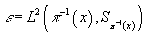
ε = L²(π^-1(X), S_π^-1(X))

of smooth spinor sections along the S¹ fiber. For x ∈ X, you have

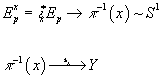
E_p^x = i_x*E_p → π^-1(X) ~S¹

π^-1(X) →Y

The assumption that Ker D_Y/X is a vector bundle on X implies that there is no spectral flow for the family of Dirac operators on the fibers D_Y/X. This means that there are no anomalies in this situation. Therefore, the adiabatic limit of the eta invariant on Y has a closed formula given by

[limit of t → ∞] [η bar] (D_V(a)⁺) = ∫_X [A hat] (R^X) ∧ [η hat]_V(a) + [η bar] (D_X ⊗ ker D_Y/X) + ½h’

where [A hat](R^X) is the [A hat] invariant polynomial applied to the curvature, ½h’ is a spin cobordism invariant, and the eta-form is a differential form on X given by

[η hat]_V(a) = 1/[squareroot of π] ∫₀^∞ tr^even [(D_Y/X + c(T)/4u) e^-(B_u)2] du/2u^½

where

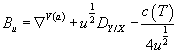
B_u = ∇^V(a) + u^½ D_Y/X – c(T)/4u^½

is the Bismut superconnection, where c is the Clifford multiplication, and T is the torsion of the connection. The eta-form is of even degree, and can be divided into homogenous even parts as

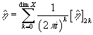
[η hat] = [summation over k from 0 to dim X] 1/(2πi)^k [η hat]_2k

and has the η-invariant of the Dirac operator along the fiber for the 0-form component.

This form comes from the spectral correction to the families version of the Atiyah-Patodi-Singer nonlocal elliptic boundary problem. Remember that Z is a disk bundle over X, where the boundary is the circle bundle Y over X. The Bismut-Cheeger-Dai theorem then says

ch(Ind(D_Z/Y)) = ∫_D [A hat] (R^Z/X) ∧ [η hat]_V(a) + (boundary correction) ∈ H^even(X, R)

where D is the disk which is the fiber of Z, D_Z/X is the family of twisted Dirac operators along the fibers of Z that are parametrized by X with the Atiyah-Patodi-Singer boundary conditions, and R^Z/X is the curvature of the vertical tangent bundle on Z. The differential

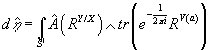
d[η hat] = ∫_S¹ [A hat] (R^Y/X) ∧ tr (e^{-(1/2πi)RV(a)})

is closed, not exact, and represents the odd Chern class of D_Y/X, R^Y/X is the curvature of the connection of the vertical tangent bundle Y, and R^V(a) is the curvature of the unitary connection on V(a). After integrating over the fiber, you get an odd degree differential form on X. This implies that the higher spectral flow vanishes.

Let’s look at the following diagram.

Compare to the similar diagram I gave earlier. A. Adams and J. Evslin suggested that the E₈ bundle in M-theory can be related to an LE₈ bundle in Type IIA on X. Starting from the principle E₈ bundle over Y, the dimensional relation of M-theory to Type IIA gives a LE₈ bundle P’ in ten dimensions characterized by the 3-form

H₃ = ∫_S¹ G₄

Remember I gave the following diagram

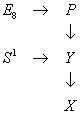
The following diagrams are related.

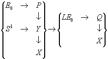
Notice that since E₈ is an approximate K(Z, 3) up to dimension 14, it follows that principle E₈ bundles over Y are classified by H⁴(Y, Z). Specifically, the characteristic class of an E₈ bundle is the restriction of the first Pontryagin class p₁ to the 4-spheres in the 4-skeleton of the base manifold.

G₄ = λ(p₁) ∈ H⁴(Y, Z)

Then the class on LE₈ is

π_*λ(p₁) ∈ H³(X, Z)

There exists a LE₈ bundle, unique up to isomorphism, such as the Diximier-Douady class

DD(LE₈) = π_*λ(p₁)

For m ∈ X, π^-1(m) = S¹, you have

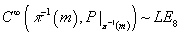
C^∈(π^-1(m), P |_π^-1(m)) ~ LE₈

This gives the fibration above with

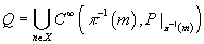
Q = [union over m ∈ X] C^∞(π^-1(m), P |_π^-1(m))

So DD(Q) = π_*λ(p₁) = H₃. The obstruction to lifting the LE₈ bundle Q to an [LE₈ hat] bundle P’ covering Q is the Diximier-Douady class.

Such a lift is possible only when H₃ = dB₂. Therefore, in the presence of F₀, only the trivial case, in the sense of the NS 3-form, can be seen in the loop picture.

Before I described how you can derive a 4-form F₄ on X from a 4-form G₄ on Y. Remember that F₂ = dA, and considering the inhomogeneous even degree form F = F₂ + F₄ + F₆ + F₈ where F₈ = _*10F₂ and F₆ is obtained from dimensional reduction G₇ = _*G₄. F is d – H closed. Then using the fact that the twisted Chern character

ch_H : K⁰(X, H) → H^even(X, H)

is an isomorphism over the reals, you get an element

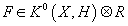
F ∈ K⁰(X, H) ⊗ R

We don’t know at this time how to lift this to a class in K⁰(X, H).

When you have branes and H-flux, the RR fields F are determined by the twisted K-theory classes x &isin K(X, H), and by the twisted Chern map

F(x)/2π = ch_H(x) [squareroot of [A hat](x)] ∈ H^[dot](X, H)

where [A hat] is the A-roof genus. It turns out that the conjugate of x, [x bar] ∈ (X, -H)

F([x bar])/2π = ch_-H [squareroot of [A hat](x)] ∈ H^[dot](X, -H)

Setting

F = [summation over n from 1 to 4] F_2n

for the gauge field strengths, the RR field equations of motion can be written as

dF = H₃ ∧ F

In order to make the RR field strengths homogeneous of degree zero, you can use K-theory with coefficients in

K(p⁺) ⊗ R[[u, u^-1]]

Where the inverse Bott element u ∈ k²(pt) has degree 2, and looks at the corresponding Chern character as a homomorphism of Z-graded rings.

ch : K(X, H) → H^even(X, H; R[[u, u^-1]]

Then the total RR field strength is written as

F = F₀ + u^-1F₂ + u^-2F₄ + u^-3F₆ + u^-4F₈ + u^-5F₁₀

In other words, the RR field equations of motion on the level of differential forms says that the RR fields determine elements in the twisted cohomology H^[dot](X, H). At the level of cohomology, this implies

H₃ ∧ F_n = 0

In K_H, or actually the Atiyah-Hirzebruch spectral sequence (AHSS), this becomes

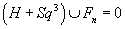
(H + Sq³) ∪ F_n = 0

Diaconescu, Moore, and Witten conjecture that the M-theory partition function on a circle bundle can be written in terms of fields satisfying the above equation.

The cup product pairing in twisted K-theory with the standard index pairing of elements of K-theory with the Dirac operator explains the upper horizontal arrows in the diagram.

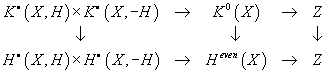
The bottom horizontal arrows are cup product in the twisted cohomology followed by cup product by [A hat](X) and by integration. By the Atiyah-Singer index theorem, the above diagram commutes. Therefore, the normalization given to the Chern character in the definition of F(x)/2π makes the pairings in twisted cohomology isometric.

Witten pointed out that the self-duality _*F = F is more subtle than that. It turns out it’s not possible to impose a classical quantization law on the periods of the self-dual p-form. This is because you can’t simultaneously measure anticommuting periods, which are the ones where the intersection number is nonzero. The way around this is to interpret the self-duality as a statement in the quantum theory and the sum over half the fluxes, meaning over a maximum set of commuting periods. Therefore, we need a phase space in the twisted K-theory with a polarization or Lagrangian subspace that naturally splits the forms in half. The lattice is

Γ_KH = K(X, H)/K(X, H)_tors

This is isomorphic to the image of the modified Chern character homomorphism of Z₂-graded rings.

[squareroot of [A hat](X)] ∧ ch_H : K(X, H) → H^even(X, H; R)

where the kernel is K(X, H)_tors, the torsion subgroup. The lattice is unimodular by Poincare duality in twisted K-theory.

To summarize, you can relate the fields of M-theory to those of Type IIA in the large volume limit, for a nontrivial circle bundle, and in the presence of nontrivial NS flux H₃. You can derive the RR fields of Type IIA from the M-theory 4-form G₄ satisfying Maxwell-like equations. Those fields are elements in twisted cohomology H^even(X, H₃).

Up until this point, we’ve been discussing the relationship between K-theory and string theory, specifically using K-theory to classify D-brane charges. One problem with that is that Diaconsecu, Moore, and Witten pointed out that the twisted K-theory classification is not compatible with the S-duality covariance in Type IIB string theory. For this reason, Hisham Sati and Igor Kriz proposed that instead of twisted K-theory, Type IIB string theory should instead be classified by elliptic cohomology. Therefore, for the remainder of this paper, I’m going to shift gears, and discuss the relation between elliptic cohomology and string theory. First I have to explain what elliptic cohomology is. Elliptic cohomology is a Taylor expansion of the formal group laws of an elliptic curve over a commutative ring. An elliptic curve is a type of cubic curve whose solutions are confined to a region of space that is topologically equivalent to a torus. The Weierstrass elliptic function p(2; g₂, g₃) describes how to get from this torus to the algebraic form of an elliptic curve. Formally, an elliptic curve over a field K is a nonsingular cubic curve in two variables f(X, Y) = 0, with a K-rational point, which may be at infinity. The field K is usually taken to be the complex numbers, C, reals, R, rationals, Q, algebraic extensions of Q, p-adic numbers, Q_p, or a finite field. By an appropriate change of variables, a general elliptic curve over a field, with a field characteristic not 2 or 3, is a general cubic curve

Ax³ + Bx²y + Cxy² + Dy³ + Ex² + Fxy + Gy² + Hx + Iy + J = 0

where A, B, C,…,J are elements of K, and can be written in the form y² = x³ + ax + b where the right hand side has no repeated factors.

Any elliptic curve not of characteristic 2 or 3 can also be written in Legendre normal form

Y² = x(x – 1)(x – λ)

If K has field characteristic three, it can be written as y² = x³ + Ay² + Bx + C. If K has field characteristic two, it can be written in Weierstrass form y² + Ay = x³ + Bx² + Cxy + Dx + E. An elliptic curve of form y² = x³ + n, where m is an integer, is called a Mordell curve.

An elliptic curve is a doubly periodic function with periods 2ω₁ and 2ω₂ such that

F(z + 2ω₁) = f(z + 2ω₂) = f(z)

which is analytic and has no singularities except for poles in the finite part of the complex plane. The half-plane ratio τ = ω₂/ω₁ must not be purely real, because if it is, the function reduces to a singly periodic function if τ is rational, and a constant if τ is irrational. ω₁ and ω₂ are labeled such that I[τ] = I[ω₂/ω₁] > 0, where I[z] is the imaginary part. A cell of an elliptic function is defined as a parallelogram region in the complex plane in which the function is not multi-valued. Elliptic functions obey the following properties.

1. The number of poles in a cell is finite.

2. The number of roots in a cell is finite.

3. The sum of complex residues in any cell is zero.

4. Liouville elliptic theorem – An elliptic function with no poles in a cell is a constant.

5. The number of zeroes of f(z) – c, called the order, equals the number of poles of f(z).

6. The simplest elliptic function has order two, since a function of order one would not have a simple irreducible pole, which would need a nonzero residue, which would violate property 3.

7. Elliptic functions with a single pole of order two with a complex residue zero are called Weierstrass elliptic functions. Elliptic functions with two simple poles having residues a₀ and –a₀ are called Jacobi elliptic functions.

8. Any elliptic function is expressible in terms of either Weierstrass elliptic functions or Jacobi elliptic functions.

9. The sum of the affixes of roots equals the sum of affixes of poles.

10. An algebraic relationship exists between any two elliptic functions with the same periods.

The elliptic functions are inversions of the elliptic integrals. The two standard forms of these functions are Jacobi elliptic functions and Weierstrass elliptic functions. Jacobi elliptic functions arise as solutions to differential equations of the form

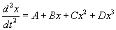
dx²/dt² = A + Bx + Cx² + Dx³

and Weierstrass elliptic functions arise as solutions to differential equations of the form

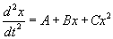
d²x/dt² = A + Bx + Cx²

The reason for the name “elliptic” is because elliptic functions generalize the trigonometric functions from circles to ellipses. Elliptic curves show up in many branches of mathematics, such as Wiles’ proof of Fermat’s Last Theorem. Elliptic curves are also important in the Monster Moonshine Conjecture, or Monstrous Moonshine. What’s amazing is that in 2007, Edward Witten related Monstrous Moonshine directly to string theory. Witten actually used the Monster group to calculate the entropy of black holes, and got results consistent with Hawking’s semiclassical approximation, but I don’t want to get too far away from the subject of this paper.

A formal group law is a formal power series behaving as if it were the product of a Lie group. They were first defined in 1946 by S, Bochner. Formal group laws are intermediate between Lie groups and Lie algebras. A one-dimensional formal group law over a commutative ring R is a power series F(x, y) with coefficients in R such that

1. F(x, y) = x + y + terms of higher degree

2. Associativity – F(x, F(y, z)) = F(F(x, y), z)

The simplest example is the additive formal group law F(x, y) = x + y. The basic idea is that F should be something like the formal power series expansion of the product of a Lie group where we choose coordinates so that the identity of the Lie group is the origin.

More generally, an n-dimensional formal group law is a collection of n power series F_i(x₁, x₂,…x_n, y₁, y₂,…y_n) in 2n variables such that

3. F(x, y) = x + y + terms of higher degree

4. Associativity – F(x, F(y, z)) = F(F(x, y), z)

where F = (F₁, F₂,…F_n), x = (x₁, x₂,…x_n), etc.

The formal group law is called commutative if F(x, y) = F(y, x). One dimensional formal group laws are usually commutative. They are commutative unless the ring r contains a nonzero nilpotent torsion element. You don’t have to have an axiom analogous to the existence of an inverse for groups since it turns out that this follows automatically from the definition of a formal group law. In other words, you can always find a unique power series G such that F(x, G(x)) = 0. A homomorphism from a formal group law F of dimension m to a formal group law G of dimension n is a collection f of n power series in m variables such that

G(f(x), f(y)) = f(F(x, y))

A homomorphism with an inverse is called an isomorphism. An isomorphism with f(x) = x + higher degree terms is called a strict isomorphism. Two formal group laws with an isomorphism between them are essentially the same. They differ only by a change of coordinates.

Here I’ll list some examples of formal group laws.

1. The additive formal group law

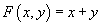
F(x, y) = x + y

2. The multiplicative formal group law

F(x, y) = x + y + xy

This rule can be understood as follows. The product G in the multiplicative group of the ring R is given by G(a, b) = ab. If we change coordinates to make zero the identity by putting a = 1 + x, b = 1 + y, and G = 1 + f, then we find that F(x, y) = x + y + xy. Over the rational numbers, there is an isomorphism from the additive formal group law to the multiplicative formal group law, given by e^x – 1. Over a general commutative ring R, there is no such homomorphism since defining it requires non-integer rational numbers, and the additive and multiplicative formal groups laws are usually not isomorphic.

3. More generally, you can construct a formal group law of dimension n from any algebraic group or Lie group of dimension n, by taking coordinates at the identity and writing down the formal power series expansion of the product map. The additive and multiplicative formal group laws obtained in this way form the additive and multiplicative algebraic groups. Another important special case of this is the formal group law of an elliptic curve.

4. The formal group law

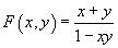
F(x, y) = (x + y)/(1 – xy)

coming from the addition formula for the tangent function

tan(x + y) = F(tan(x), tan(y))

5. The formal group law

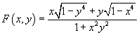
F(x, y) = (x[squareroot of (1 – y⁴)] + y[squareroot of (1 – x⁴)])/(1 + x²y²)

is a formal group law over Z[½] found by Euler, in the form of the addition law for an elliptic integral.

Any n-dimensional formal group law gives an n-dimensional Lie algebra over the ring R, defined in terms of the quadratic part F₂ of the formal group law

[x, y] = F₂(x, y) – F₂(y, x)

The natural functor from the Lie groups or algebraic groups to Lie algebras can be factorized into a functor from the Lie groups to formal group laws, followed by taking the Lie algebra of the formal group law.

Lie groups → Formal group laws → Lie algebras

Over fields of characteristic zero, formal group laws are essentially the same as finite dimensional Lie algebras. The functor from finite dimensional formal groups laws to finite dimensional Lie algebras is an equivalence of categories. Over fields of non-zero characteristic, formal group laws are not equivalent to Lie algebras. Sometimes, when you go from an algebraic group to its Lie algebra, you lose too much information, but if you go to the formal group law, you keep enough information. Therefore, you can use formal group laws as a substitute for Lie algebras if the characteristic is not zero.

Let’s say that f is a homomorphism between one-dimensional formal group laws over a field with characteristic p > 0. Then f is either zero or the first non-zero term in its power series expansion is

ax^ph

for some non-negative integer h, called the height of the homomorphism f. The height of the zero homomorphism is defined to be infinity. The height of a one-dimensional formal group law over a field of characteristic p > 0 is defined to be height of its pth power map. Two one-dimensional formal group laws over an algebraically closed field of characteristic p > 0 are isomorphic if and only if they have the same height, which can be any positive integer or infinity.

1. The additive formal group law F(x, y) = x + y has height h = ∞, since its pth power map is 0.

2. The multiplicative formal group law F(x, y) = x + y + xy has height h = 1, since its pth power map is (1 + x)^p – 1 = x^p.

There is a universal commutative one-dimensional formal group law over a universal commutative ring defined as follows. Let’s say

F(x, y) = x + y + Σ c_{i, j}xⁱx^j

For indeterminate c_{i, j}, and we define the universal ring R to be the commutative ring generated by the elements c_{i, j} with the relations that are forced by the associative and commutative laws. For any commutative ring S, one-dimensional formal group laws over S correspond to ring homomorphisms from R to S. The commutative ring R is called Lazard’s universal ring. You might think it would be very complicated, but actually Lazard proved that it has a very simple structure. It is just a polynomial ring over the integers on generators of degrees 2, 4, 6,…, where c_{i, j} has degree 2(i + j – 1). The reason for the strange grading is that Quillen proved that the coefficient ring of complex cobordism is naturally isomorphic as a graded ring to Lazard’s universal ring.

Let’s say Z_p is the ring of p-adic integers. The Lubin-Tate formal group law is the unique one-dimensional formal group law F such that e(x) = px + x^p is an endomorphism of F.

e(F(x, y)) = F(e(x), e(y))

More generally, you can allow e to be any power series such that e(x) = px + higher degree terms, and e(x) = x^p mod p. All the group laws for different choices of e satisfying these conditions are strictly isomorphic. For each element a in Z_p, there is a unique endomorphism f of the Lubin-Tate formal group law such that f(x) = ax + higher degree terms. This gives an action of the ring Z_p on the Lubin-Tate formal group law. There is a similar construction with Z_p replaced by any complete discrete valuation ring with finite residue class fields. The Lubin-Tate formal group laws were introduced by Jonathan Lubin and John Tate as part of their successful effort to isolate the local field part of the classical theory of complex multiplication of elliptic functions.

Now I’m going to try to explain elliptic cohomology. I just need to discuss some more preliminary things. An R-valued genus μ is a ring homomorphism

μ : Ω_so → R

from the bordisms ring

Ω_so = (closed oriented manifolds)/(cobordisms)

to R. The product in Ω_so is the Cartesian product of manifolds, and the sum is the disjoint union of manifolds. Genera appear as indices of Dirac operators, and are related to the cohomologies of points.

1. The Euler characteristic X → χ(X), which is the index of D = d + d* under the grading by form degree, is close to being a genus, but is not corbordism invariant.

2. The signature genus is the index of D = d + d*, but under the grading of differential forms as positive or negative, according to the signature of the bilinear form

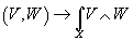
(V, W) → ∫_X V ∧ W

3. The [A hat]-genus is the index of a Dirac operator coming from a spinor bundle.

4. The elliptic genus has been interpreted non-rigorously by Witten as the index of a Dirac operator, which is the heterotic string supercharge, on loop space.

Let’s say A is any abelian group. Given a topological space X, there are several equivalent ways to define the nth singular cohomology group

Hⁿ(X, A)

with values in A. One way is to say that this group equals that of homotopy classes of maps from X to the space K(A, n), which is defined to have all homotopy groups trivial except for the nth one, which is isomorphic to A.

Hⁿ(X, A) ~ [X, K(A, n)]

For this reason, K(A, n) represents ordinary cohomology. It is a simple fact that the based loop space K(A, n) is homotopy equivalent to K(A, n – 1).

ΩK(A, n) ~ K(A, n – 1)

A list

E = (E_n)_{n ∈ N}

of topological spaces such that each space is the loop space of the next one

ΩE_n ~ E_{n – 1}

is called a spectrum. The sequence E_n = K(A, n) is called the Eilenberg-MacLane spectrum, which represents ordinary cohomology. Stated this way, the definition of generalized cohomology is obvious. A generalized cohomology is a collection of functors

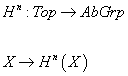
Hⁿ : Top → AbGrp

X → Hⁿ(X)

From topological spaces to abelian groups, which is represented by a spectrum E = (E_n)

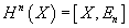
Hⁿ(X) = [X, E_n]

The first interesting example of a generalized cohomology theory, right after ordinary cohomology, is K-theory.

X → K_n(X)

A well-known result by Atiyah says that K₀ is represented by the space Fred(H) of Fredholm operators on some separable Hilbert space H.

K(H) ~ [X, Fred(X)]

Some generalized cohomologies have special properties. In particular, we are used to there being a graded ring structure on the cohomology groups, given by the cap product for ordinary cohomology, and by the tensor product of vector bundles for K-theory. It is clear that in order for

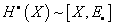
H^[dot](X) ~ [X, E_[dot]]

to be a ring, the spaces E_[dot] need to have a ring-like structure themselves. Since everything is defined only up to homotopy, there is freedom in having this ring structure defined only up to higher coherent homotopy. There is one natural choice for how to deal with these higher coherencies.

A spectrum E which is a graded ring

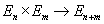
E_n x E_m → E_{n + m}

in this higher coherent sense is called an E_∞-ring spectrum, or simple an E_∞-ring.

An elliptic curve over a field k is the collection of solutions in k x k to an equation in k of the form

f(x, y) = Ax³ + Bx² + Cx + D – y² = 0

where A, B, C, D ∈ k are constants defining an elliptic curve. For the present purpose, the single most important property of an elliptic curve

S = {(x, y) ∈ k x k | f(x, y) = 0}

is that it is naturally equipped with an abelian algebraic group structure S x S → S. Elliptic curves over the complex numbers are precisely the same thing as Riemann surfaces of genus 1, and hence the same as one-loop string diagrams. This makes it quite possible that elliptic curves play a central role in a cohomology theory which assigns to a point in the space of 2dSCFT, the corresponding 1-loop partition function.

We are interested in a 2-dimensional field theory with N = (1, 0) superconformal symmetry, which is the heterotic string. We could also work with Type II superstrings, but these would yield less cohomological information.

There is a graded Hilbert space H of states, which we can think of as something like the space of sections of a spinor bundle over free loop space. Represented on H is the Laplace-like operator

Δ = L + [L bar]

and an operator

P = i(L – [L bar])

which generates rigid rotations of the parametrization of the loops. The chiral combinations

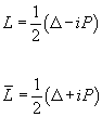
L = ½(Δ + iP)

[L bar] = ½(Δ – iP)

are the zero-modes of the two Virasoro algebras. Let’s say there is an N = (n, m) supersymmetry, essentially up the fact that we’re considering only zero-modes, if there are n mutually graded commuting odd-graded generators G⁽ⁱ⁾ such that

L = (G⁽ⁱ⁾)²

and m mutually graded commuting odd-graded operators [G bar]⁽ⁱ⁾ such that

[L bar] = ([G bar]⁽ⁱ⁾)²

Restricting to N = (1, 0), you have a single odd-graded operator G with L = G². We want something like the index of this G. For ordinary supersymmetric quantum mechanics, you compute the index by means of the partition function over a circle of length t, which turns out to be independent of t. Here we compute the partition function over a torus of length t and twist s by

ind_WittenG = str(e^-tΔ e^-sP)

ind_WittenG = str(q^L [q bar]^{[L bar]})

where

q = e^{-(t + is)}

[q bar] = e^{-(t – is)}

Since L = G² is the square of an odd operator, the usual argument applies, and we see that this partition function localizes on the kernel of L

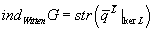
ind_WittenG = str([q bar]^{[L bar]} |_{ker L})

You can simplify this further by splitting the supertrace into contributions coming from the eigenspaces

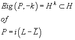
Eig(P₁ – k) = H^k ⊂ H of P = i(L – [L bar])

ind_WittenG = [summation over k &isin Z] (q^k) sdim(ker ∩ H^k)

This power series in q is the index of the loop space operator. If you had used N = (1, 1) supersymmetry, the remaining sum would have localized itself on the kernel of [L bar] and collapsed to a mere integer.

ind_WittenG is a weak integral modular form, which means that

1. It is a holomorphic function f on the upper half plane.

2. It has the transformation property

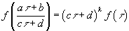
f((aτ + b)/(cτ + d)) = (cτ + d)^kf(τ)

for all elements of SL₂(Z)

3. Only finitely many terms for negative powers of k are nonvanishing.

4. All coefficients are integers.

All weak integral modular forms are combinations of

1. The discriminant

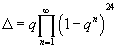
Δ = q[product series over n from 1 to ∞] (1 – qⁿ)²⁴

2. The two Eisenstein series

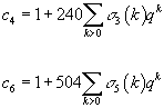
c₄ = 1 + 240[summation over k > 0] σ₃(k)q^k

c₆ = 1 – 540[summation over k > 0] σ₅(k)q^k

where

σ_r(k) = Σ_{d | k} dr

The ring of weak integral modular forms, MF_* is

MF_* = Z[c₄, c₆, Δ, Δ^-1]/(c₄³ – c₆² – (12)³Δ)

The index of an ordinary Dirac operator takes values in the integers, which is the K-theory of a point. The index of a Dirac operator on loop space takes values in the ring MF_* of weak integral modular forms. This lives in something like the elliptic cohomology of a point. The generalized cohomology appearing here comes from an E_∞-spectrum called topological modular forms, or tmf.

Let’s say H is some multiplicative generalized cohomology, such as the one coming from an E_∞-ring spectrum. You have the graded ring associated by H to the space

K(Z, 2) ~ CP^∞ ~ PU(H) ~ BU(1)

Since BU(1) is the classifying space for U(1)-bundles, the ordinary cohomology group H^[dot](BU(1), Z) is the ring freely generalized over Z by Chern class c of the universal line bundle U(H) → PU(H). Under the tensor product of two line bundles L₁ → X and L₂ → X, their Chern classes simply add up in ordinary second cohomology.

c₁(L₁ ⊗_X L₂) = c₁(L₁) + c₂(L₂)

This particular property turns out to be modified for generalized cohomology theories. They will have other group laws, different from the simple one on the right hand side of the above equation. Let’s say H is any generalized cohomology theory. Its value on BU(1) is always a power series ring

H^[dot](BU(1)) = H^[dot](pt)[[t]]

over a single generator t of degree 2 with coefficients in the cohomology ring of a point. Remember that t is itself a class of a map

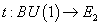
t : BU(1) → E₂

if E is the spectrum representing the generalized cohomology.

Given any complex line bundle on some space X, classified by the class of the map φ : X → BU(1), you can pull back the generator t along this map to obtain an element of H^[dot](X).

φ*t : X →^φ BU(1) →^t E₂

Notice that for ordinary cohomology, this is precisely the pullback of the universal first Chern class along φ to X, hence the Chern class c₁(L) = φ*t of our complex line bundle on X. For generalized cohomologies φ*t is no longer the Chern class of our line bundle. It is instead the generalized Chern class. The whole point of this exercise is that we can now in principle compute how these generalized Chern classes of complex line bundles behave under the tensor product operation of line bundles. They will, in general, unlike the ordinary Chern class, not just add up. For instance, for K-theory, you get the following group law

c₁(L₁ ⊗_X L₂) = c₁(L₁) + c₁(L₂) + c₁(L₁)c₁(L₂)

More generally, you find

c₁(L₁ ⊗_X L₂) = f(c₁(L₁), c₂(L₂))

where

F(t₁, t₂) ∈ H^[dot](pt)[[t₁, t₂]]

is any formal power series with coefficients in the cohomology ring of a point satisfying the following three axioms.

1. identity – f(x, 0) = f(0, x) = x

2. commutivity – f(x, y) = f(y, x)

3. associativity – f(x, f(y, z)) = f(f(x, y), z)

Such a power series is called a commutative one-dimensional formal group law over the ring H^[dot](pt). Under suitable assumptions, over an algebraically closed field, there are only three types of one-dimensional algebraic groups corresponding to three types of formal group laws.

1. The additive group law – x . y = x + y

2. The multiplicative group law – x . y = x + y + xy

3. A group law defined by an elliptic curve.

An elliptic cohomology is any generalized cohomology whose formal group law, which governs the generalized Chern classes of tensor products of complex line bundles, is given by an elliptic curve. So there are many elliptic cohomology theories. You can do something like taking the direct limit over all of these. The result is represented by an E_∞-spectrum called tmf. Its value over a point is the ring of weak integral modular forms that arise as the partition function of heterotic strings.

The Weierstrass form of an elliptic curve E is an equation in two variables x and y of the form

y² + a₁xy + a₃y = x³ + a₂x + a₄y + a₆

If the determinant Δ of E is nonvanishing, it is a smooth curve. Thinking of the above equation as living over the real numbers, such smooth curves are certain smooth curves in R². Straight lines in R² which coincide with this curve in three points P, Q, and R define an abelian group structure on points by setting

P + Q + R = 0

For many applications, it is convenient to perform a coordinate transformation from (x, y) to (w, z) with

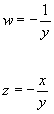
w = -1/y

z = – x/y

Then there is an f such that the above equation for the elliptic curve reads equivalently

w = f(z, w)

By iteratively reinserting f into itself according to this equation, you get

f(z, w) = z³(1 + A₁z + A₂z² + …)∈ Z[a₁, a₂, a₃, a₄, a₆] [[z]]

which is a power series in z starting in degree 3, with coefficients being polynomials in the a’s, over the integers. Using this, you can understand the above addition on the elliptic curve as given by a power series in two variables. Specifically, if (w₁, z₁) and (w₂, z₂) are two points on the smooth elliptic curve E, which means that the z coordinate is determined by w, then the result of adding them has a z-coordinate which is given by the power series

F_E(z₁, z₂) ∈ Z[a₁,…a₆][[z₁, z₂]]

This F_E is a formal group law, which implies

1. F(z₁, 0) = z₁

2. F(z₁, z₂) = F(z₂, z₁)

3. F(F(z₁, z₂), z₃) = F(z₁, F(z₂, z₃))

for all z_j. From this you can show that inverses of all elements exist.

The most famous example of such a formal group law is obtained from taking a one-dimensional real Lie group, looking at the tangent space T_e at a given point e, using the exponential map to identify a neighborhood of e in the group with the tangent space, and expanding for all x, y ∈ T_e the multiplication in the group as

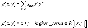
μ(x, y) = Σ_{n, m} a_{n, m}xⁿy^m

μ(x, y) = x + y + higher terms ∈ R[[x, y]]

In general, formal groups are local expansions of group laws. The power series F_E associated with a smooth elliptic curve as described above is the expansion of the additive group law defined by the elliptic curve.

Quillen explained that formal groups are related to complex cobordisms. Let MU_* be the complex cobordism ring, which is the ring whose elements are cobordism classes of stably complex manifolds with multiplication being the Cartesian product, and addition being a disjoint union.

Ω_*^U = MU_*

This ring is universal for formal group laws in the sense that there is a formal group law

F_MU

over MU_* such that for every formal group law F over any ring R, there is a unique ring homomorphism

θ : MU_* → R

such that

F = θ_*F_MU

which means that if

F_MU(x, y) = Σ_{n, m} a_{n, m}xⁿym

then

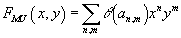
F(x, y) = Σ_{n, m} θ(a_n, a_m)xⁿy^m

Remember that every elliptic curve E gives rise to a formal group law F_E over the ring Z[a₁,…a₆]. You find that for every elliptic curve, there is a unique ring homomorphism

θ_E : MU_* → Z[a₁,…a₆]

Using this homomorphism, you get an action MU_* on Z[a₁,…a₆]. We want to use this to form a generalized cohomology theory by tensoring Z[a₁,…a₆] with the universal cohomology MU_* theory defined by complex cobordisms.

Let’s set MU_n(X) to be the ring of maps

φ : Mⁿ → X

from stably complex n-manifolds Mⁿ to X, where we identify two maps if their domain manifolds are cobounded by a stably complex (n + 1)-manifold, where stably complex means that you can embed Mⁿ in some R^N for sufficiently large N, such that the normal bundle Mⁿ in R^N is a C-vector bundle. The entire ring MU_*(X) is just the direct sum

MU_*(X) = ⊕_n MU_n(X)

and in particular, the bare MU_* from above is shorthand for the MU-cohomology of a point

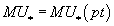
MU_* = MU_*(pt)

It is important for the following construction that there is a natural graded action MU_*(pt) on any MU_*(X)

MU_n(pt) x MU_m(X) → MU_{n + m}(X)

simply given by taking a map

Mⁿ → pt

and

M^m → X

and forming the obvious map

Mⁿ x M^m → pt x M ~ X

Therefore, you have an action of the ring MU_*(pt) both on the ring Z[a₁,…a₆] and on the ring MU_*(X) for all X. Therefore, for each elliptic curve E and space X, you can form the graded ring

E_*(X) = MU_*(X) ⊗_MU*(pt) Z[a₁,…a₆]

This is the elliptic cohomology ring of X with respect to the elliptic curve E. From this, you can recover ordinary integral cohomology and K-theory as degenerate cases of elliptic cohomology. If the elliptic curve is

y² = x³

with a bad singularity at (0, 0), the corresponding group law is simply

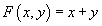
F(x, y) = x + y

This is the group law which corresponds to ordinary integral cohomology.

The elliptic curve

y² = x³ + x²

has a singularity which is not quite as bad. It gives rise to the group law

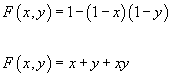
F(x, y) = 1 – (1 – x)(1 – y)

F(x, y) = x + y + xy

This is the group law which corresponds to complex K-theory.

A special case of elliptic curves are the Jacobi curves, which are of the form

y² = 1 – 2δx² + εx⁴

depending on the two parameters δ and ε. The discriminant is

Δ = ε(δ² – ε)²

Using

g₂ = (δ² – 3ε)/3

g₃ = δ(δ² – 9ε)/27

You can also write

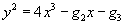
y² = 4x³ – g₂x – g₃

which only works in characteristic > 3. The formal group law corresponding to these curves is

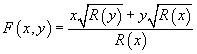
F(x, y) = (x[squareroot of R(y)] + y[squareroot of R(x)])/R(x)

where

R(x) = 1 – 2δx² + εx⁴

This formula was originally discovered by Euler although he didn’t call it a formal group law. You can write F(x, y) as

F(x, y) = g^-1(g(x) + g(y))

where

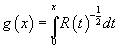
g(x) = ∫₀^x R(t)^-½dt

Now, let [M tilde]_* be the ring of modular forms under the subgroup of SL(2, Z) generated by

τ → τ + 2

τ = -1/τ

There is a theorem by Landweber, Ravenel, and Stong which says that for δ and ε algebraically independent over Q, you have

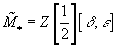
[M tilde]_* = Z[½][δ, ε]

and for all the rings in the diagram

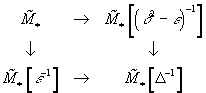
there exist a generalized homology theory h_* such that h_*(pt) is that given ring. This is constructed by noticing that the formal group law defines an action of the oriented cobordism ring on the given ring R_* from above, which allows us to form the homology ring of some space x as

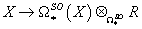
X → Ω_*^SO(X) ⊗_Ω*^SOR

A genus is a ring homomorphism

φ : Ω_*^SO → Λ

from oriented cobordisms to any other ring Λ that is also a Q-algebra.

Since

Ω_*^SO ⊗ Q ~ Q[[CP²], [CP⁴],…]

it’s sufficient to specify φ on [CP²ⁿ]. The following expression

G_φ(x) = ∫₀^x [summation over n ≥ 0] φ [CP²ⁿ] t²ⁿ dt = [summation over n ≥ 0] φ [CP²ⁿ] (x^{2n + 1}/(2n + 1))

is called the logarithm of the genus. Ochanine defined a genus to be elliptic if this logarithm is of the form

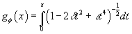
g_φ(x) = ∫₀^x (1 – 2δ t² + ε t⁴)^-½dt

for suitable ring elements δ and ε, algebraically independent over Q and Δ ≠ 0.

There is a theorem by Landweber, Ochanine, and Stong which says that if a genus φ is elliptic, then its image is

φ(Ω_*^SO) = Z[δ, 2γ, 2γ², …2γ²ⁿ]

where

γ = (δ² – ε)/4

Furthermore, the image of its spin cobordism is

φ(Ω_*^spin) = Z[16δ, (8δ)², ε]

Here are some examples.

1. ε = δ = 1

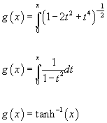
g(x) = ∫₀^x (1 – 2t² + t⁴)^-½dt

g(x) = ∫₀^x 1/(1 – t²) dt

g(x) = tanh^-1(x)

This corresponds to the signature genus or L-genus.

2. ε = 0, δ = -1/8

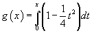
g(x) = ∫₀^x (1 – ¼t²)^-½dt

This corresponds to the [A hat]-genus. As Atiyah and singer found with their famous index theorem, for M compact and dim M = 2n, the [A hat]-genus

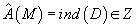
[A hat](M) = ind(D) ∈ Z

is the index of a Dirac operator on M, taking values in the integers.

We want to lift this statement to the loop space of M. It turns out that this is possible if M is string, which means, according to a theorem by Laughlin, that its first two Stieffel-Whitney classes, and one half of the first Pontryagin class, vanishes. In this case, there is something like a Dirac operator on loop space LM, and there is a theorem by Witten and Zagier which says that its index is a genus which is the q-series of a modular form, called the Witten genus, which is the partition function of the heterotic string.

Topological modular forms, or tmf, are like the universal elliptical cohomology. The way elliptic cohomology was defined above depended on the choice of coordinates, in the Weierstrass form, for an elliptic curve. In a vague sense, tmf is the coordinate-free version of elliptic cohomology. The Weierstrass form

y² + a₁xy + a₃y = x³ + a₂x² + a₄x + a₆

is invariant under the coordinate transformations of the form

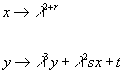
x → λ² + r

y → λ³y + λ²sx + t

where λ is an invertible unit.

Call this group of transformations G. Let

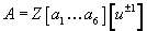
A = Z[a₁,…a₆][u^±1]

and form the cohomology theory

X → (E_A)(X) = MU_*(X) ⊗_MU*A

Then, according to a theorem by Hopkins, Miller, and Goerss, which has been given a more conceptual proof by Jacob Lurie, the G-invariant part (E_A)^G of E_A is a model for tmf. There is a map from the tmf cohomology of a point to modular forms

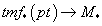
tmf_*(pt) → M

whose kernel and cokernel are annihilated by 24. It is known that

tmf_*[1/6][pt] = Z[1/6, c₄, c₆] = M_*[1/6]

The Witten genus is the composition map

M_string → tmf → KU[[q]]

From string cobordisms over tmf to power series in q with coefficients in K-theory.

The term “elliptic cohomology” was first introduced in 1986 by P. S. Landweber, D. C. Ravenel, and R. E. Stong to designate a cohomology theory obtained by tensoring the oriented cobordism theory with a ring of modular forms in characteristic ≠ 2. Since then, numerous publications have appeared. They attempt to connect elliptic cohomology to other generalized cohomology theories, such as Morava’s K-theories. They also attempt to give a geometric interpretation of elliptic cohomology. Despite many very interesting results, there seems to be no consensus on what exactly is the elliptic cohomology. However, the situation is well-understood outside the prime 2. Here, I will describe the Landweber-Ravenel-Stong theory. Let’s say Ω_*^SO is the oriented bordism theory with coefficient ring Ω_*^SO, and let

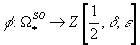
φ : Ω_*^SO → Z[½, δ, ε]

be the level 2 elliptic genus with logarithm

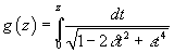
g(z) = ∫₀^z dt/[squareroot of (1 – 2δt² + εt⁴)]

The ring

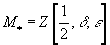
M_* = Z[½, δ, ε]

is a ring of level 2 modular forms in characteristic ≠ 2, and can be viewed, via φ, as an Ω_*^SO-module. It also has a natural grading for which deg δ = 2, and deg ε = 4.

Let π ∈ M_* be any homogenous element of positive degree. Then the functor

X → Ω_*^SO(X) ⊗_Ω*^SOM_*[π^-1]

is a positive homology theory called elliptic homology, with a coefficient ring M_*[π^-1].

A similar construction using oriented cohomology leads to a multiplicative periodic cohomology theory called elliptic cohomology. The proof of this theorem was first given by Landweber, Ravenel, and Stong under the assumption that π is one of the factors of Δ = ε(δ² – ε)², and was based on Landweber’s Exact Functor Theorem, and also interesting congruencies for Legendre polynomials. The general form stated above is due to Jens Franke who showed that the exactness of the functor is a consequence of a theorem by Deuring and Eichler saying that the height of the formal group of an elliptic curve in positive characteristic is always 1 or 2.

A 1-dimensional commutative formal group law (FGL) over a commutative ring R is a series

F(x, y) = x + y + Σ a_ijxⁱy^j ∈ R[[x, y]]

which satisfies

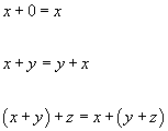
x + 0 = x

x + y = y + x

(x + y) + z = x + (y + z)

The significance in homotopy theory is as follows. We call a ring-valued generalized cohomology theory E complex-oriented if the canonical complex line bundle γ over CP^∞ is E-oriented, meaning it satisfied an E-Thom isomorphism. A choice of such isomorphism is called a complex orientation of E. It follows that every complex bundle is E-oriented. Furthermore, the complex orientation determines a Chern class of complex bundles precisely analogously as in the case of ordinary cohomology. The way FGL’s enter the picture is that there exists a unique FGL over the ring E_*, depending only on E and complex orientation, such that for complex line bundles L and M over a space X

c₁(L ⊗ M) = c₁(L) ⊗ c₁(M)

If you change the complex orientation on E, the formal group law gets replaced by a strongly isomorphic formal group law G which means that there exists a formal series

f(x) = x + a₂x² + a₃x³ + …∈ E_*[[x]]

such that

f(x) + f(y) = f(x + y)

The formal group law up to strong isomorphism is a powerful invariant of a complex-oriented generalized cohomology theory. The FGL of ordinary cohomology is additive. F(x, y) = x + y. The FGL of K-theory is multiplicative. F(x, y) = x + y + v₁xy, where v₁ is the Bott element. Over a Q-algebra, all FGL’s are isomorphic, just as all rational cohomology theories are equivalent. There is a universal formal group law, which is a commutative ring L with a formal group law F such that for any commutative ring R and any formal group law G on R, there is a unique homomorphism of rings L → R, which carries F to G. This ring was discovered by Lazard. Then Quillen discovered that surprisingly L is isomorphic to the ring of coefficients of MU, complex cobordism which is in some sense the universal complex-oriented generalized cohomology theory.

If we localize at prime p, then MU breaks up as a direct sum of certain theories called BP. There is a corresponding notion of p-typical FGL. The coefficients of BP are

BP_* = Z[v₁, v₂, v₃,…]

dim(v) = 2pⁿ – 2

The formal group law on BP_* was also first observed in algebra, and is due to Cartier. By work of Baas-Sullivan, it is possible to create generalized cohomology theories at will by killing regular sequences in the ring BP_* and/or inverting elements in its coefficient ring. This leads to a menagerie of generalized cohomology theories. Some of the important theories and their coefficients are

1. Johnson-Wilson theory BP(n)

Z[v₁, v₂,…v_n]

2. Landweber theory E(n)

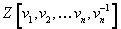
Z[v₁, v₂,…v_n, v_n^-1]

3. Integral Morova K-theory [K tilde](n)

Z[v_n, v_n^-1]

4. Morova K-theory K(n)

Z/p[v_n, v_n^-1]

5. Connective Integral Morova K-theory [k tilde](n)

Z[v_n]

6. Connective Morova K-theory k(n)

Z/p[v_n]

Some of these theories have interesting formal group laws. For instance, the formal group law on K(n)_* has height n which means

[p]_Fx = x + _F +…+_Fx = v_nx^pn

Studying isomorphisms of this FGL led Lubin and Tate to the discovery of the Lubin-Tate FGL on the ring

W_n[[a₁, a₂, …a_{n – 1}]][u, u^-1]

where W_n is the ring of Witt vectors, which are integers of an Eisenstein extension of order pⁿ of the field of p-adic numbers Q_p. The Lubin-Tate coefficient ring turns out to be a completed sum of copies of E(n)_*, and you can consider a generalized cohomology theory with the Lubin-Tate coefficient ring, which is essentially a completed sum of E(n). Lubin-Tate laws were not invented for homotopy theory, but instead for algebraic number theory.

For n = 2, you can also consider cohomology theories whose formal group laws are elliptic, meaning they are obtained by Taylor expansion of the formal group law on an elliptic curve over some commutative ring. Such theories are called complex-oriented elliptic cohomology theories. Ande, Hopkins, and Strickland defined a 2-periodic ring spectrum as a generalized cohomology theory E with an orientation of the identical complex line bundle on CP^∞, which, when restricted to CP¹ has an inverse on E_*. If in addition, E_{2n + 1} = 0 for all n, an evenness condition, and there is an elliptic curve [curly E] over E_* with an isomorphism of its formal group law with the formal group law of E, which is the elliptic spectrum. The word “spectrum” is s term of algebraic topology which means a generalized cohomology theory. The reason for using a separate word is that spectra may be refined to a category which contains a rigid point set level information, analogous to point set level maps of spaces. Cohomology theories see only maps up to homotopy. The rigid level is necessary for certain more complicated constructions such as simplicial realizations.

The elliptic spectrum

E_* = Z[a₁, a₂, a₃, a₄, a₆][u, u^-1]

is associated with the Weierstrass curve

y² + a₁uxy + a₃u³y = x³ + a₂u²x² + a₄u⁴x + a₆u⁶

where dim(x) = 4, dim(y) = 6. The map

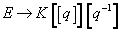
E → K[[q]][q^-1]

for this spectrum can be constructed using the Tate parametrization

σ_k(n) = Σ_{d | n} d^k, a_k = Σ_{n > 0} σ_k(n) qⁿ

You can define the above map by

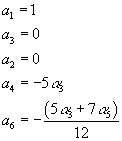
a₁ = 1

a₂ = 0

a₄ = -5α₃

a₆ = -(5α₃ + 7α₅)/12

The coefficients of a₆ turn out to be integers.

At the same time, the Lubin-Tate spectrum

E_* = W₂[[a]][u, u^-1]

is also an elliptic spectrum. Its corresponding elliptic curve is

y² + auxy + u³ = x³

To construct the map

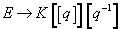
E → K[[q]][q^-1]

in this case, where the target is K-theory with coefficients in W₂, the Lubin-Tate FGL is

[2]_Fx = (2x) + _F(aux²) + _F(u³x⁴)

and Lubin-Tate theory implies that over a ring where au is invertible, this is isomorphic to a multiplicative FGL. Therefore, we define the map by

au = v₁

u = v₁q^-1

or equivalently

a = q

u = v₁q^-1

we get the correct map after composition with the automorphism of

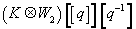
(K ⊗ W₂) [[q]][q^-1]

which sends the formal group law to a multiplicative FGL of K-theory.

y² + auxy + u³y = x³

is a Weierstrass curve with

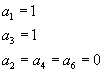
a₁ = 1

a₃ = 1

a₂ = a₄ = a₆ = 0

However, the map for this theory is not the same as the map coming from the Tate parametrization, thus further confirming the nonuniqueness of the coordinates. Another disadvantage of the theory is that the character map requires you to use

K ⊗ W₂

and thus the Chern character requires crystalline cohomology.

Now, we are finally in a position to use elliptic cohomology to describe superstring theory and M-theory. It might turn out to be more appropriate to use elliptic cohomology than K-theory. There are two superstring theories with two supersymmetries in ten dimensions. One is nonchiral N = (1, 1) Type IIA theory, and the other is chiral N = (2, 0) Type IIB theory. Their fields fall into two sectors, the Ramond-Ramond (RR) sector, and the Neveu-Schwarz (NS) sector. The RR fields naturally couple to D-branes of even spatial dimension in Type IIA. The RR fields naturally couple to D-branes of odd spatial dimension in Type IIB. The NS fields couple to NS-branes. The classification of RR fields has been an active area of research. The charges can be classified, in the absence of NS fields, by K-theory of spacetime. The RR charges are classified by K⁰(X) in Type IIB, and by K¹(X) in Type IIA. The RR fields are classified by K¹(X) for Type IIB, and by K⁰(X) for Type IIA. In the presence of a NS B-field, or its field strength H₃, the relevant K-theory is twisted K-theory. Freed, Witten, and Kapustin showed by analysis of wordsheet anomalies for the case of the NS field

[H₃] ∈ H³(X, Z)

is a torsion class, and by Bouwknegt and Mathai for the non-torsion case. Other versions of K-theory are relevant to string theory. KO and KSp theories are relevant for Type I, equivariant K-theory for orbifolds, and Antiyah’s Real K-theory for orientifolds.

Eleven-dimensional M-theory has four BPS objects, which are the membrane M2, the fivebrane M5, the Kaluza-Klein monopole MKK, and the gravitational wave MW. Compactification on a circle leads to Type IIA. The objects in the theory, such as the M-branes, reduce to Type IIA D-branes. D-branes and M-branes can have anomalies associated with them. This prevents the existence of nonzero or well defined partition functions. For the M5-brane, the partition function is nonzero if the M5-brane can be decoupled from the bulk, including the M2-brane. In Type IIA, the D-brane anomaly cancellation is the vanishing of the third integral Stiefel-Whitney class W₃. In the presence of a NS field, it becomes

[H₃] – W₃ = 0

This can be interpreted in the context of twisted K-theory Atiyah-Hirzebruch spectral sequence (AHSS) as the vanishing of the third differential. This contains a topological part W₃, and twisting part, which is the NS 3-form H₃.

There is another anomaly found by Diaconescu, Moore, and Witten in the context of relating the K-theory of ten-dimensional spacetime X of Type IIA to the partition function of M-theory on an eleven-dimensional manifold Y in the topological sector captured by an E₈ gauge theory. This anomaly is an obstruction to the partition function being well-defined. The condition is the vanishing of the seventh integral Stiefel-Whitney class W₇ of X, considered as the base space of a circle bundle with total space Y. The anomaly still persists in twisted K-theory.

A completely different motivation is to what extent K-theory can describe D-branes, and in particular, the fields and charges, and whether you should seek alternatives in some cases where K-theory breaks down or does not see the whole picture. For instance, on Calabi-Yau spaces, you could use the derived category of sheaves, or the presence of an NS field, the derived category of twisted sheaves. The advantage of using the derived category description of D-branes instead of K-theory is that it contains far more data which specifies the D-brane. On non-geometric backgrounds, such as discrete torsion D-branes, there is a search for a quantum K-theory, such as possibly R/Z generalized cohomology theory. It is natural then to suspect that on general topological spaces, an alternative to K-theory is needed, such as to describe phenomena at strong coupling and at the quantum level, perhaps more “M-theoretic” in nature.

One promising candidate for describing the M-theory partition function is elliptic cohomology. First of all, you might wonder if there is a twisting part that can be added to the topological part W₇ in analogy to H₃ in the brane anomaly. The immediate candidate would be the Hodge dual H₇ = _*10H₃ of H₃. You might wonder whether W₇ analogously comes from a differential of degree 7, d₇ in AHSS. However, K-theory AHSS of a 10-dimensional Spin manifold, d₇ is zero. W₇ can not possibly come from K-theory AHSS. However, it turns out that it does come from d₇, not in K-theory AHSS, but rather in Morova K-theory and elliptic cohomology. The vanishing of the Diaconescu-Moore-Witten obstruction W₇ = 0 is precisely equivalent to orientability of the Spin manifold X with respect to complex oriented elliptic cohomology. This is a generalized cohomology theory which in addition to the Bott periodicity element v₁, contains another periodic element v₂ of dimension 6. Furthermore, v₂ is invertible in elliptic cohomology while v₁ is not. Is there an analog of the M-theory partition function based on elliptic cohomology instead of K-theory? If so, what additional physical information does it contain? Is elliptic cohomology, rather than K-theory, the right tool for describing the path from Type IIA to M-theory?

It now appears that the elliptic cohomology based partition function may be more closely tied to M-theory than the K-theory partition function. For one thing, you can see directly that the elliptic partition function, when it exists, is not anomalous. The distinction between existence and lack of anomaly may seem trivial, but the point is that in the K-theory case, there is a condition of vanishing of a certain quadratic function on torsion. This leads to W₇ = 0. In elliptic cohomology, W₇ = 0 is a condition for orientability, but when satisfied, there is no other condition on torsion. In addition, in elliptic cohomology, you have

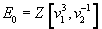
E = Z[v₁³, v₂^-1]

so the partition function can be thought of as a family of partition functions indexed by a parameter v₁³v₂^-1. What is the physical meaning of these additional modes? The interpretation of v₂ as an element in the 6-dimensional complex cobordism group suggests that these modes are related to interactions between an M2-brane and an M5-brane. Out of the many possible configurations allowed by supergravity, we think the right ones are intersections between an M2-brane and an M5-brane on a string, which, in the S¹-compactified case, connects with the fundamental Type IIA string. Furthermore, this suggests that the theory can be H₇-twisted, specifically when the M5-brane is not complex-oriented. Even in the untwisted case, we see an anomaly of such states when w₄ ≠ 0.

We also thin that the non-invertibility of the Bott element in elliptic cohomology is related to the disappearance of some of the RR charges when we pass from Type IIA to M-theory. These charges can be constructed from each other in any theory in which the Bott element is invertible.

First, I will briefly review Diaconescu-Moore-Witten M-theory. M-theory is defined on a circle bundle Y with Type IIA on the base space X. In M-theory, there is an E₈ bundle associated to it, with the p₁/2 class λ. In Type IIA, there are RR fields which are reductions of that class, and are classified by twisted K-theory. First, let’s look at the M-theory side compactified to X. Stong has shown that

[Ω tilde]₁₀^Spin(K(Z, 4)) = Z₂ x Z₂

This implies that there are two independent Z₂-valued invariants of the pair (x, a) where

a ∈ H⁴(X, Z)

They are

1.

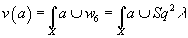
v(a) = ∫_X a ∪ w₆ = ∫_X a ∪ Sq²λ

where the second integral is due to X being spin. This is a linear function.

v(a + b) = v(a) + v(b)

2. In 8k + 2 dimensions, index D_vR is a topological invariant mod 2,

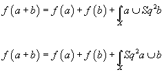
f(a + b) = f(a) + f(b) + ∫_X a ∪ Sq²b

f(a + b) = f(a) + f(b) + ∫_x Sq²a ∪ b

where f(a) is not a linear function. The form

Q(a, b) = f(a + b) – f(a) – f(b)

is a homomorphism from

Ω₁₀(K(Z, 4) x K(Z, 4))

to Z₂. Q vanishes if either a or b is zero. This implies that Q is a homomorphism to Z₂ of the relative bordism group

Ω₁₀^Spin(K(Z, 4) x K(Z, 4), K(Z, 4) x {*} x {*} x K(Z, 4))

which Diaconescu, Moore, and Witten calculated to be Z₂. One of them is

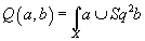
Q(a, b) = ∫_X a ∪ Sq²b

which is nonzero, such as on

X = S² x S² x CP³

Now let’s say a is a torsion class. Then Q(a, b) is a torsion pairing

T : H_tors^k(X, Z) x H_tors^{n – k + 1}(X, Z) → U(1)

This is because

β(Sq²b) = Sq¹Sq²b = Sq³b

by Adem relations. Now sq³b is a torsion class, and so

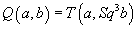
Q(a, b) = T(a, Sq³b)

The partition function vanishes unless Q = T = 0. This implies the condition Sq³λ = 0. Therefore, M-theory on a spin manifold of the form X x S¹ is inconsistent if W₇ = 0.

On the Type IIA side, the relevant calculations are K-theory calculations. Remember that we have the mod 2 index I(v) of the Dirac operator with values in a real vector bundle V. For v ∈ KO(X), you can define the mod 2 index I(v) of the Dirac operator with values in v. For any x ∈ K(X), you have

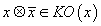
x ⊗ [x bar] ∈ KO(X)

so you can define

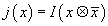
j(x) = I(x ⊗ [x bar])

Define the Z₂-valued function

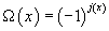
Ω(x) = (-1)^j(x)

which satisfies

Ω(x + y) = Ω(x)Ω(y)(-1)^{ω(x, y)}

where

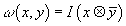
ω(x, y) = I(x ⊗ [y bar])

is an integer-valued unimodular antisymmetric bilinear form on the lattice

Γ = K(X)/K(X)_tors

Now, if Ω(x) = 1 for torsion elements K(X), then it can be regarded as a function of Γ, and so can be used to define the line bundle, and therefore its section, the RR partition function. If Ω(x) ≠ 1 on K(X)_tors, then the partition function of the theory vanishes upon summing over torsion. It’s similar for twisted K-theory, for

Γ_H = K(X, H)/K(X, H)_tors

Then, in 2003, Diaconsecu, Moore, and Witten showed that the M-theory anomaly and Type IIA are related in a one-to-one fashion.

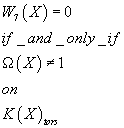
W₇(X) = 0 if and only if Ω(X) ≠ 1 on K(X)_tors

In 1999, Daniel S. Freed and Edward Witten showed that an anomaly in D-branes is given by

W₃ + [H₃] = 0

where W₃ is the integral class, obtained from the second mod 2 Stiefel-Whitney class, w₂, by the Bockstein homomorphism. A D-brane can’t wrap a submanifold of X unless the Poincare dual can be lifted to K-theory. The anomaly comes from the fact that when this condition is not satisfied then you can have other branes ending on the one you are talking about so you can’t view it in isolation, so the partition function is not well-defined.

At the level of AHSS, it is the third differential d₃ = W₃ + [H₃]. At the level of the full twisted K-theory, you should solve the extension problem, and this could be an obstruction to a K-theory lift. For a compact manifold X, this is an obstruction to being Spin^c. However, there is another way of looking at it, in terms of the K-theory AHSS differential. A Spin^c-manifold would be K-theory orientable, and so would have a K-theory homology fundamental class. Now, you can see directly that if W₃ ≠ 0, then X has no K-theory fundamental class.

Stiefel-Whitney classes are conjugates of Steenrod operations by the Thom isomorphism. However, you can also look at this in terms of Poincare duality. Assuming X is 10-dimensional, let’s say

α ∈ H⁷(X, Z)

is a class such that W₃α ≠ 0. Then

Sq³α ≠ 0

The Milnor primitives Q, invented by J. Milnor in 1958, are elements of the Steenrod algebra of dimension 2^{i + 1} – 1, and

Sq3 = Q₁

where Q is the primary differential d₃ in the K-theory AHSS. So you see that

d₃(α)= u

in the K*-AHSS where

U ∈ H¹⁰(X, Z)

is the dual of the fundamental class. Dualizing, we conclude that the fundamental class X does not lift to K-theory homology, so X is not K-theory orientable.

Next, we’ll discuss W₇. This is not the 7th Stiefel-Whitney class

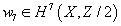
w₇ ∈ H⁷(X, Z/2)

which always vanishes for a spin manifold. Instead,

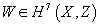
W ∈ H⁷(X, Z)

is a canonical integral of w₇, specifically

β(w₆)

where

β H^k(X, Z/2) → H^{k + 1}(X, Z)

is the Bockstein homomorphism. The fact that the mod 2 reduction w₇ of W₇ vanishes signifies the fact that W₇ is divisible by 2 in integral cohomology.

This is analogous to another situation. For a spin manifold X, the first Pontryagin class p₁ is divisible by 2 and λ = p₁/2 is an obstruction to what is called string structure. You might wonder if there is any connection between these two things. One connection is that string structure is the same as thing as lifting the structure group of the tangent bundle on X to a 2-connected cover String(10) of Spin(10).

However, because of Bott periodicity, this is the same thing as the 6-connected cover since there are no homotopy groups between them. In other words, the classifying map X → BSpin(10) lifts to BString(10), which is 7-connected, and there is no cohomology in dimension 7. Therefore, W₇(X) = 0. You have w₆ = Sq²λ so λ = 0 implies w₆ – 0, which implies W₇ = 0. However, it is not true that W₇(X) = 0 implies p₁(X)/2 = 0. For instance, for X = S² x S² x CP³, p₁/2 is nonzero but there is no odd cohomology, so W₇ = 0.

You might wonder what is the geometric meaning of W₇ ≠ 0. Remember the definition of Stiefel-Whitney classes. If you denote the Poincare duality by

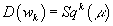
D(w_k) = Sq^k(μ)

where

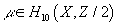
μ ∈ H₁₀(X, Z/2)

is the fundamental class. Remember the actions of the Steenrod operations on homology.

Sq^k : H_m(X, Z/2) → H_{m – k}(X, Z/2)

You therefore have

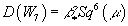
D(W₇) = β_*Sq⁶(μ)

where

β_* : H_m(X, Z/2) → H_{m – 1}(X, Z)

is the Bockstein.

Now, there is an integral cohomology operation

[Q tilde]₂ : H^m(X, Z) → H^{m + 7}(X, Z)

which is dual to a homological operation lowering the dimension by 7, and which is the integral lift of the Milnor primitive Q₂. Furthermore, the operation [Q tilde]₂ is closely tied to a generalized cohomology theory [K tilde](2) called p = 2 integral second Morova K-theory, which is a reduction of elliptic cohomology. You have

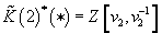
[K tilde](2)*(*) = Z[v₂, v₂^-1]

where v₂ is of dimension 6. The way this theory is tied to [Q tilde] is as follows. For every generalized cohomology, there is a corresponding generalized homology theory. There are Atiyah-Hirzebruch spectral sequences both in homology and cohomology.

Working in homology, the AHSS for [K tilde](2) is

E_pq² =H_p(X, [K tilde](2)_p(*)) → [K tilde](2)_pq(X)

The dimensions imply that possible differentials of this AHSS are d^{6k + 1}. The connection with [Q tilde]₂ is that

D⁷ = [Q tilde]₂

Now, [Q tilde]₂ coincides with βSq⁶ modulo elements of lower Cartan-Serre filtration. There are only three linearly independent Steenrod operations in dimension 6, which are

Sq⁶

Sq⁵Sq¹

Sq⁴Sq²

By Adem relations, you have

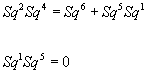
Sq²Sq⁴ = Sq⁶ + Sq⁵Sq¹

Sq¹Sq⁵ = 0

On the fundamental scale

μ ∈ H₁₀(X, Z)

The last two must vanish by the assumption that X is a spin manifold.

We conclude that

[Q tilde]₂(μ) = βSq⁶(μ) = D(W₇)

Therefore, you see that W₇ ≠ 0 if and only if the primary differential in the homology [K tilde](2)-AHSS for X is nonzero on μ, which in turn happens if and only if X is not [K tilde](2)-orientable, as any higher differentials are out of filtration degree range. We have therefore proved that a 10-manifold X is orientable with respect to [K tilde](2) if and only if W₇(X) = 0.

It is natural to conjecture that [K tilde](2) can be replaced by elliptic cohomology E. This is in fact true as can be proved by more technical manipulation of the AHSS. Of course, you have to decide which definition of E you want to choose. You can get some insight from looking at the characteristic classes. Notice that W₇ = 0 for any compact complex 10-dimensional manifold, so you should use complex oriented elliptic cohomology. However, the Hopkins-Miller universal elliptic cohomology theory tmf is MO<8>-orientable, which means that every manifold whose stable normal bundle has structure group String = O<8> is tmf-orientable. Therefore, we have an explanation of the above distinction between the p₁/2 and W₇ obstructions. It signifies a connection between M-theory and elliptic cohomology but not tmf.

Now, there are still various models for complex-oriented cohomology E which are characterized by their coefficient rings. Under the assumption that the associated elliptic curve must allow both multiplicative and p = 2-singular reduction, these theories contain equivalent homotopical information but each has advantages and disadvantages. Choosing a complex-oriented elliptic cohomology is like choosing coordinates. The problem is there is no universal complex-oriented elliptic cohomology theory. There is a universal generalized elliptic curve, called the Weierstrass curve

y²x + a₁xyz + a₃y³ = x³ + a₂x²z + a₄xz² + a₆x³

over the ring

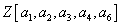
Z[a₁, a₂, a₃, a₄, a₆][u, u^-1]

and you can choose

E_* = Z[a₁, a₂, a₃, a₄, a₆][u, u^-1]

This theory is still not universal because of automorphisms. However, the parameters a_i are generalized modular forms, and there is a character map

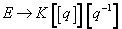
E → K[[q]][q^-1]

where K is K-theory, q is the parameter of dimension 0, K[[q]] is therefore a product of infinitely many copies of K, and [q^-1] means that q is inverted.

You can simplify is you complete at prime 2. If you choose

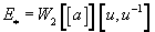
E_*= W₂[[a]][u, u^-1]

where W₂ is a ring of Witt vectors, such as the ring of integers, of the extension of the field Q₂ of 2-adic numbers by an Eisenstein polynomial of degree 4, dim(a) = 0, dim(u) = 2. This theory’s formal group law, calculating

c₁(ξ ⊗ η)

from c₁(ξ), c₁(η) for line bundles ξ, η, is a Lubin-Tate law F₂ of height 2. You can construct a character map for this theory, except that k must be replaced by K-theory with coefficients in W₂.

You can simplify it further if you notice that the cohomology theory E with

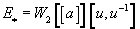
E_* = W₂[[a]][u, u^-1]

is a completion of a finite sum of suspensions of copies of the cohomology theory E(2) which has

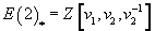
E(2)_* = Z[v₁, v₂, v₂^-1]

where v₁ has dimension 2, and v₂ has dimension 6.

For instance, you can set v₂ = u³, v₁ = au. This cohomology theory lacks some of the manifest modular symmetries of the other elliptic cohomology theories, such as being 6-periodic in dimension, but has the simplest coefficients.

We are dealing with Spin manifolds, so you need a real form EO(2) of elliptic cohomology, which is obtained by taking the fixed point cohomology theory of E under Z/2-action which comes from the FGL isomorphism –i(X), where i(X) is the inverse series of F₂. It’s difficult to make this definition precise since you have to prove the Z/2-action is rigid, and not just up to homotopy. We’ll assume X is orientable under EO(2).

The main point of the construction of the RR partition function of Type IIA D-branes is the function Ω, which is equivalent to j, defined on K⁰(X). From homotopy theory, the construction of j means that for x ∈ K⁰(X), the virtual bundle x ⊗ [x bar] has a real structure, and therefore represents an element of KO⁰(X). The mod 2 index is simply the Kronecker product with the KO-orientation KO-homology class μ ∈ KO₁₀(X)

KO⁰(X) ⊗_KO* KO₁₀(X) → KO₁₀(*) = Z/2

The construction of the partition function fails when this index is nonzero on torsion elements x ∈ K⁰(X).

Now, let’s try to do the same thing with elliptic cohomology. We’ll deal directly with the generalized cohomology class, specifically with E⁰(X)-classes. The manifold X is E-orientable, so it has an orientation class [x]_E ∈ E₁₀X. For x, y ∈ E⁰(X), you have

ω(x, y) = {x[y bar], [x]_E} ∈ E₁₀ = E₀

Now, you need an elliptic refinement of the function j. Assuming that X is EO(2)-orientable, you have an EO(2)-orientation class [x]_EO(2) ∈ EO(2)₁₀(X). Now, for x ∈ E⁰(X), the class x[x bar] lifts canonically to EO(2)⁰(X), so you can put

j(x) = {x[x bar], [x]_EO(2)} ∈ EO(2)₁₀

To see what the right hand side is, you have to compute EO(2)₁₀. It makes the computation easier to reduce E to a theory E(2) with coefficients

Z₂[v₁, v₂, v₂^-1]

It is a direct summand of E so this allows you to leave out repeating terms. You also have the twist. The way you should view the real version of the theory E(2) is as a Z/2-equivariant generalized cohomology theory called ER(2). Cohomology classes of such theories are indexed by k + lα, where α denotes the sign representation of Z/2. The orientation class of X is in ER(2)₁₀(X) so the Kronecker product lies in ER(2)₁₀(*).

This group is a Z/2-vector space with basis

v₁³ⁿv₂^{2 – n}σ^-4a²

n ≥ 1

where v₁ has dimension 1 + α, v₂ has dimension 3(1 + α), σ has dimension α -1, and a has dimension -α, so the generators have dimension 10. Therefore, you have an element

j(x) ∈ Z/2[v₁³, v₂^-1] = EO(2)₁₀

You have to make sense of the identity

j(x) + j(y) – j(x + y) = ω(x, y) mod 2

This is more difficult than the K-theory case since we do not have index-theorectical arguments for E(2), and both sides of the above equation appear to belong to different generalized cohomology groups. However, you can use a purely homotopy-theoretical argument. The left hand side of the above equation is

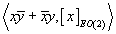
{x[y bar] + [x bar]y, [x]_EO(2)}

while the right hand side is

{x[y bar], [x]_E(2)}

Therefore, all you have to do is make sense of

{a + [a bar], [x]_EO(2)} = {a, [x]_E(2)} mod 2

for any

a ∈ E(2)⁰(X)

You need the transfer map

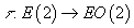
τ : E(2) → EO(2)

This can be interpreted as a map on fixed points of the Z/2-equivariant generalized cohomology theories

ER(2) ∧ (Z/2₊) → ER(2) ∧ (EZ/2₊ →^N F(EZ/2₊, ER(2))

where EZ/2 is a contractible space with free Z/2-action. The second arrow N is the norm map from a Borel homology to Borel cohomology theory.

For a ∈ E(2)⁰(X), you have the following commutative diagram.

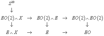
The unlabeled arrows are forgetful maps and multiplications. This diagram sows that the above equation is valid if we map the right hand side to the left hand side using the transfer. In 2001, P. Hu and Igor Kriz showed that the norm map can be calculated by dividing by σa the differential in the Tate cohomology spectral sequence for

[ER hat]

which crosses the line between Borel homology and cohomology. The relevant differential is

d : σ^-2 → v₁a³

so you get

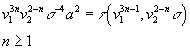
v₁³ⁿv₂^{2 – n}σ^-4a² = τ(v₁^{3n – 1}, v₂^{2 – n}σ^-5)

n ≥ 1

Now, I’m going to show how elliptic cohomology is related to M-theory. Let’s say you have a 10-dimensional compact Spin manifold X, and put Y = X x S¹. Elliptic cohomology of X and Y are related by the Kunneth theorem

E*(Y) = E*(X) ⊗_E* E*(S¹)

so

Eⁿ(Y) = Eⁿ(X) ⊕ E^{n – 1}(X)

Let’s say the background is twisted by an NS 3-form H-field. In that case, you must replace K-theory by twisted K-theory. However, C. L. Douglas pointed out that twistings of K-theory determine topological modular forms. Specifically, twistings of K-theory are classified by the space BGL₁(K), and you have a map BGL₁(K) → tmf. Therefore, twistings of K-theory are encoded in tmf, which then maps into E. Therefore, while in twisted K-theory, you must change the theory with each H-field. Elliptic cohomology unifies all of these twisted cases into one theory. This might be because of the connection between elliptic cohomology and 2-vector bundles.

While K-theory twistings give rise to topological modular forms, complex-oriented elliptic cohomology plays a more basic role. This should allow twisting by the field strength H₇, which is the field strength associated with the NS 5-brane, similar to how H₃ is associated with the fundamental string F1. The lift to M-theory of the NS-branes leads to M-branes. The fundamental string expands in one dimension along the M-theory circle to become the M2-brane, while the NS 5-brane lifts to an M5-brane, thus maintaining the same worldvolume dimension. The reason for this difference in codimension in the lifting is because of the dimensions of the relevant forms. In 10 dimensions, the NS field strengths have dimensions three and seven, while in 11 dimensions, the fields have dimensions four and seven. Witten showed that in the case Y = X x S¹, a match between the partition function of M-theory calculated from the G₄-field, which is the field strength associated with the M2-brane, and the Type IIA partition function, which is calculated from the fundamental string RR sector. When increasing the coupling in Type IIA, you get M-theory, compactified on X x S¹, and the fundamental string gets another dimension, and is then identified with the M2-brane. This suggests that the elliptic refinement of the partition function reflects interaction between an M2-brane and M5-brane. The M5-brane is an object in M-theory with electromagnetically dual coupling to the field strength G₄. In Type IIA, it loses a dimension, and becomes a D4-brane. However, using strong-weak duality, you can identify the M5-brane with a 6-dimensional object which is the NS5-brane in Type IIA, which couples magnetically to the NS charge.

Let’s say W is the worldvolume of the NS5-brane. Then the fundamental class κ ∈ H₆ must satisfy

Sq³(κ) = 0 ∈ H₃(X, Z)

meaning that κ must lift to the K-theory homology of x. This is also d³ in the E(2)-homology AHSS of X. However, the next differential d⁵ is in homological dimension 1, and therefore is excluded, so κ lifts to a class in E(2)₆(X). Now, by multiplying by the elliptic cohomology element v₂^-1, which is of dimension 6, you get an element of E(2)₀(X). It turns out that 6 is the only dimension of a worldvolume ≤ 10 which can be shifted to 0 by inverting the element v₂. Notice that, unlike in K-theory, the Bott element v₁ is not inverted in elliptic cohomology. This may be singling out the 5-brane as the object whose interactions give the main part of the M-theoretic correction to the Type IIA partition function. In M-theory, the M5-brane couples magnetically to the field strength G₄. In Type II superstring theory, RR D-branes of lower dimension can be generated from higher dimension by tachyonic condensation. This involves the Gysin isomorphism or the Bott element. In M-theory, not all even dimensions are allowed. Specifically, you can not reverse the process, and for instance, turn a 2-brane into a 4-brane in M-theory. This seems to be related to the non-invertibility of the element v₁ in elliptic cohomology.

What might be the twisting with respect to the field strength H₇? Notice that v₂ ∈ MU_* is represented by a complex manifold called a Milnor manifold whose Segre characteristic number is 2. However, an M5-brane, while it must be orientable, may not be a complex manifold. Therefore, it is reasonable to propose the inclusion of such non-complex M5-branes will introduce a new twisting. Elliptic cohomology has the formal group law of an elliptic curve. Therefore, you should be able to see the group, or possibly subgroups of, SL(2, Z). Since the modular parameters that appear in M-theory and string theory are usually of the form

τ = (field) + i(volume modulus)

it seems reasonable to propose the moduli in the form

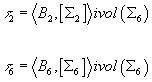
τ₂ = {B₂, [Σ₂]} + ivol(Σ₆)

τ₆ = {B₂, [Σ₆]} + ivol(Σ₆)

where < , > is the Kronecker product, [ ] is the fundamental class, Σ₂ is a two-cycle that can correspond to F1, and Σ₆ is a six-cycle that can correspond to NS5.

The modular parameter τ₆ should be related to the map

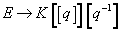
E → K[[q]][q^-1]

by an equation which we can schematically write as

q = e^2πiτ₆

In order to make physical predictions from this, we would need a more precise normalization of coordinates to predict the exact choice of group of modular transformations, as well as a formula for the M5-brane charge.

We still have to interpret v₂^-1v₁³. One possibility is that M2 and M5 coexist, and the membrane modulus is not inverted. If a soliton spectrum contains the M5-brane, then it automatically contains the M2-brane. This can be understood by the Hanany-Witten effect that implies that an M2-brane is created when two M5-branes intersect. Also, an M2-brane appears from the dielectric M5-branes in the limit when the 3-cycle shrinks to zero.

Next, I’ll briefly review the intersections and bound states of M-branes. M2-branes and M5-banes can consistently coexist in compatibility with the gravitational anomaly cancellation. They obey a Dirac quantization condition

eg = 2πnG_N

where e is the M2 charge, g is the M5 charge, and G_N is the 11-dimensional Newton constant. The presence of M2 and M5 modify the equation of motion to

d*G₄ = G₄ ∧ G₄ + gf₃ ∧ J₅ + eJ₈ + (2πG_n/g)X₈

where J₅ is the current Poincare dual to M5, J₈ is the current Poincare dual to M2, X₈ is the 8-polynomial associated with the gravitational anomaly, and f₃ is the M5 worldvolume field. A more detailed analysis would involve Cheeger-Simons differential characters. From supergravity, the allowed supersymmetric intersections are

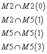
M2 ∩ M2(0)

M2 ∩ M5(1)

M5 ∩ M5(1)

M5 ∩ M5(3)

where (p) means the intersection is a p-brane. The second one is interesting since it is the intersection over a string of the two types of branes, and is one of the building blocks for brane intersections.

The reduction of the intersection M2 ∩ M5(1) along M2 leads to F1 ending on NS5, and along M5 leads to D2 ending on D4. There are many possible D-brane bound states in Type II string theory. One way they arise is by placing D-branes in a constant background B-field. The worldvolume coordinates of the Dp-brane become noncommutative (NC) along the directions of the nonvanishing B-field. If B is spacelike, you can define a decoupling limit of NCYM, which is NC field theory. If B is timelike, you get noncommutative open string theory (NCOS). In principle, any bound state in Type IIA should have a lift to M-theory. The analogous situation in M-theory would be M-branes in a constant background C-field. The configuration of M2-branes ending on M5 is the lift of strings ending on D-branes. You can also have a decoupled theory, the light Open Membrane (OM). Six-dimensional OM-theory is the high energy limit of 5-dimensional NCYM and NCOS. Compactification of OM-theory on an electric circle leads to NCOS. Compactification of OM-theory on a magnetic circle leads to NCYM. A constant background C-field is equivalent to a constant M5 worldvolume field f₃. This represents a bound state of this M5 with a delocalized M2 along 2 of the 5 spatial dimensions of M5. Many of the bound states involving different combinations can be related to (M2, M5) by a Lorentz transformation, and this seems to indicate that the latter is the basic bound state.

This suggests that you can use the IIA-side to interpret the elliptic refinement, since the G₄ approach should be exactly dual. The IIA side is easier to work with since you have the usual expansion of the radial excitation modes of the fundamental string. The meaning of the parameter v₂^-1v₁³ is that it comes from the interaction with a complex oriented M5-brane, and that the partition function should be twisted if the M5-brane if the M5-brane is not complex-oriented. Therefore, we should consider what kinds of possible bound states between M2-branes and M5-branes that you can have. one possibility is that an open M2-brane is a boundary of an M5-brane. This is suggested by the non-invertibility of v₁, and therefore v₂^-1v₁³ in elliptic cohomology. However, from the point of view of the M5-brane, it is not clear whether such states would be anomalous. Also, in the IIA-dimensional reduction, there is no direct role of the open string partition function. it may therefore be that rather than ending on the M5-brane, the M2-brane intersects the M5-brane in a fundamental string, and the elliptic partition function reflects the energy that the bound state gets from the intersection. You could also claim that just as in string theory, where open strings require closed strings, that here open membranes seem to be only needed to imply the existence of the branes, and they do not enter into the calculation of the partition function.

The elliptic refinements of the IIA partition function, or alternatively the M-theory G₄ partition function, picks up states arising from the intersection of an M2-brane with an M5-brane, which could be H₇-twisted if the M5-brane is not complex-oriented. In the present untwisted case, there is an anomaly of these states when w₄ ≠ 0. On the IIA side for Y = X x S¹, the intersection is the end of the Type IIA fundamental string. The elliptic function after suitable renormalization and computation of the 5-brane charge should compute the M2-M5 intersecting state correction to the G₄ M-theory partition function. Orientability with respect to EO(2) is equivalent to vanishing w₄. This is relevant to M-theory backgrounds as well as to the M5 anomaly. In 2000, Witten showed that G₄/2π is quantized as w₄/2 mod Z. The condition w₄ – 0 implies that there are no half-integral fluxes, which is the case for the relevant Z₂-orbifolds and orientifolds. Witten also showed that w₄ also shows up as part of the mod 2 index and therefore, the anomaly for the M5-brane.

M-theory unifies string theories, and thus is the best candidate for a quantum theory of gravity. The study of the partition function related to the four-form has uncovered deep connections to K-theory, twisted K-theory, and elliptic cohomology. The M-theory actions contains contains the usual 11-dimensional supergravity terms, which are the Einstein-Hilbert, the G₄ kinetic terms, the Rarita-Schwinger terms, as well as subtle topological terms such as the Chern-Simons term and the one-loop term given by

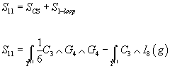
S₁₁ = S_CS + S_1-loop

S₁₁ = ∫_Y¹¹ (1/6) C₃ ∧ G₄ ∧ G₄ – ∫_Y¹¹ C₃ ∧ I₈(g)

where

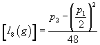
[I₈(g)] = (p₂ – (p₁/2)²)/48

written in terms of the Pontryagin classes of the tangent bundle.

Using cobordism, Witten uncovered a structure related to E₈ index theory by writing the above action on a twelve-manifold Z¹² whose boundary is the M-theory eleven-manifold Y¹¹. In twelve dimensions, the topological part of the action is then

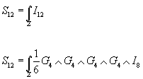
S₁₂ = ∫_Z I₁₂

S₁₂ = ∫_Z (1/6) G₄ ∧ G₄ ∧ G₄ – G₄ ∧ I₈

You have the mod 6 congruence which was derived by S. P. de Alwis using physical arguments related to Horova-Witten boundaries, and by Edward Witten using E₈ index theory.

You can write the Chern-Simons term in an exponentiated form as

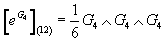
[e^G₄]₍₁₂₎ = (1/6)G₄ ∧ G₄ ∧ G₄

which looks like a character. Obviously, this encodes the correct normalization factor.

Next look at the one-loop term. The total string class is defined in terms of the individual string classes by

λ = λ₀ + λ₁ + λ₂ +…

where λ₀ = 1, λ₁ = p₁/2 is the usual string class, λ₂ = p₂/2 is the second string class, and so on. The exponentiated class or total string character is defined by

e^λ/24

whose degree eight component gives

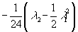
-(1/24)(λ₂ – ½λ₁²)

which is exactly the one-loop gravitational polynomial I₈, as it shows up in the action with the minus sign. This is analogous to writing the second Chern character in terms of the Chern classes as

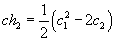
ch₂ = ½(c₁² – 2c₂)

Then the total topological action can be written as

[e^G₄[e^λ]^1/24]₍₁₂₎

the degree twelve component.

This apparently predicts a term

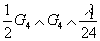
½ G₄ ∧ G₄ ∧ λ₁/24

that can be written in terms of

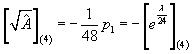
[squareroot of A hat]₍₄₎ = -(1/48) p₁ = -[e^λ/24]₍₄₎

In fact, you can ask in a different but related context if you can replace the K-theoretic formula

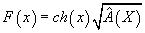
F(x) = ch(x)[squareroot of A hat(X)]

for the RR fields with something like

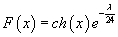
F(x) = ch(x)e^-λ/24

They match for the two lower degrees of the gravitational part, which is 0 and 4, but not the degree 8.

Anyway, you can find a rationale to exclude such terms, as well as terms containing λ₃, on the basis of parity. You want to retain terms like

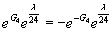
e^G₄ e^λ/24 = -e^-G₄ e^λ/24

which kills the terms with an even number of G₄‘s and keeps the ones with an odd number of G₄‘s. Therefore, the total topological action is given by the parity-odd part of the twelve-form component of the character. The Lagrangian of the 11-dimensional supergravity has a sign of the 3-form potential C₃. along with a reversal in sign of an odd number of space coordinates.

The phase of the M-theory partition function would then be written as

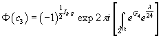
Φ(C₃) = (-1) ^½I_R.S. exp 2πi[∫_Z¹² e^G₄ e^λ/24]

where you pick the degree twelve component out of the integrand. The sign ambiguity in the phase of the Pfaffian of the Rarita-Schwinger operator is given in terms of the Rarita-Schwinger action I_R.S..

Now, we make an analogy with the construction of the Chern character based on ordinary curvatures of connection one-forms. This suggests that an analogous theory based on the Pontryagin classes or the string classes. Here is the Chern character.

ch(F₂) = e^F₂ = rk + F₂ + ½ F₂ ∧ F₂ + (1/6) F₂ ∧ F₂ ∧ F₂ + …

Now, do the same thing with G₄.

e^G₄ = c + G₄ + ½ G₄ ∧ G₄ + (1/6) G₄ ∧ G₄ ∧ G₄ + …

The Chern character should be written in terms of the Lie-algebra valued curvature, whose trace we’ve suppressed. The character corresponding to G₄ does not have a value since G₄ does not correspond to a structure group in a literal sense. If it is a 2-gerbe, then the simplest way is to take it to be abelian, and thus corresponding to a U(1). If you write the C-field in terms of the E₈ gauge fields, such as C₃ = CS₃(A), then G₄ might have some nonabelian aspect to it.

Now look at this equation.

E^G₄ = c + G₄ + ½G₄ ∧ G₄ + (1/6)G₄ ∧ G₄ ∧ G₄ + …

You can think of this as defining a sort of M-theoretic character analogous to the Chern character. Here “c” refers to the appropriate concept in this case that replaces the rank of the bundle for the case of K-theory. The E₈ and Rarita-Schwinger indices are then encoded in

Index(M object) = ∫M = ∫e^G₄

where the M objects are

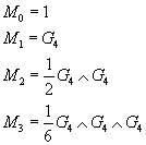
M₀ = 1

M₁ = G₄

M₂ = ½G₄ ∧ G₄

M₃ = (1/6)G₄ ∧ G₄ ∧ G₄

where M₁ corresponds to the M2-brane, M₂ corresponds to the M5-brane, or little M-theory, and M₃ corresponds to M-theory. Therefore the M-branes and M-theories are unified.

In order to be technically correct, M must also include a gravitational correction term e^λ/24. You simply replace M with

M’ = Me^λ/24

You exclude odd parity for odd-rank characters, and even parity for even-rank characters.

The Chern-Simons construction for Type IIA string theory and for M5-branes is similar. In both cases, you have a manifold of dimension 4k + 2 with k = 1 for the 5-brane, and k = 2 for the Type IIA string theory. The Chern-Simons construction requires extending the (4k + 2)-dimensional X to a (4k + 3)-dimensional manifold X × S¹, which in the case of Type IIA is just the extension to M-theory. Then the construction requires extending the resulting manifold to a (4k + 4)-dimensional coboundary N such that ∂N = X x S¹. In the case of IIA and M-theory, this is the manifold Z. In both cases, you are extending the manifold together with a four-class, so this requires the vanishing of the spin cobordism cohomology group.

MSpin_{4k + 3}(K(Z, 4))

R. E. Stong showed that this was the case for k = 2, and M. J. Hopkins and I. M. Singer showed that this was the case for k = 1. Similar to the Chern-Simons term in M-theory, you can write the corresponding quadratic term involving only G₄ on N₈ in an exponential way.

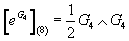
[e^G₄]₍₈₎ = ½g₄ ∧ G₄

which is the formula derived by Witten, and also in a more general situation by Hopkins and Singer. This suggests there is a generalized cohomology theory in which G₄ lives, and the character is a multiplicative map from the theory of M-objects to 4kth cohomology.

M = e^G₄ : [curly M] → H^4k

where [curly M] is the generalized cohomology theory that describes M-theory. Remember that the Chern character is a map from K-theory to even cohomology

ch : K → H^even

and satisfies for two vector bundles E and F

ch(E ⊕ F) = ch(E) ⊕ ch(F)

ch(E ⊗ F) = ch(E) ∧ ch(F)

We want the M-theory character to have properties analogous to the Chern character so we want it to satisfy

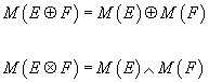
M(E ⊕ F) = M(E) ⊕ M(F)

M(E ⊗ F) = M(E) ∧ M(F)

where E and F are M-objects. Notice that dM = 0 since G₄ is closed due to the Bianchi identity.

For K-theory, the objects corresponding to the two-form curvature F₂ are vector bundles. Therefore, the corresponding M-objects related to G₄ would be 2-gerbes, 2-vector bundles, etc.

A connection on a U(1)-bundle looks locally like a 1-form, so you can integrate it along a path and compute how the phase of charged particles changes when you move it along that path.

x → y

f : x → y is a path f from point x to point y.

If you categorify this whole idea once, you get a connection that looks locally like a 2-form, called a connection on a U(1)-gerbe. This is just a gadget that you can integrate over a surface to compute how the phase of a charged string moves when you slide it along that surface.

F : f → g is a path F from the path f to the path g.

If you categorify once more, you get connection on a U(1) 2-gerbe. This is something that looks locally like a 3-form, which describes what happens when you move 2-branes around. Since 11d supergravity has a 3-form, and M-theory has 2-branes, you therefore need to categorify the concept of a U(1) bundle twice, and use 2-gerbes when discussing M-theory.

From the general structure of the M-theory character, and from the mod 24 congruence of the string class, the theory should be some form of elliptic cohomology related to topological modular forms. There should also be some relation to E₈ and Rarita-Schwinger bundles.

One way to better understand gerbes is to think of them as differential objects. You now replace local holomorphic functions h_αβγ on a complex manifold by smooth functions, and assume that the values lie in the group U(1) of unit complex numbers. There is then the idea of a unitary connection on a grebe, provided by real differential 1-forms A_αβ and 2-forms F_α such that

iA_αβ + ia_βγ + iA_γα = h^-1_αβγdh_αβγ

F_β – F_α = dA_αβ

Then

H = dF_α = dF_β

is the global closed 3-form, which is defined to be the curvature of the connection. The de Rham class

[H/2π] ∈ H³(M, R)

is integral, just as [F/2π] is the first Chern class if F is the curvature form for a connection on a line bundle. Equivalence classes of grebes with connections like these are familiar in the theory of Cheeger-Simons differential characters of degree 2.

The best known example of a grebe with connection arises when the manifold M is a compact simple Lie group G. There is a natural gerbe on G whose curvature is a multiple of the bi-invariant 3-form B(X, ([Y, Z]) where B is the killing form. For G = U(n), this is tr(g^-1dg)³. Whereas a line bundle has holonomy around a closed surface. More generally, if the curvature of a gerbe vanishes, then there is a holonomy in H²(M, U(1)). For example, B(X, [Y, Z]) vanishes on a T ⊂ G because T is abelian, so the gerbe is flat there. It is a rather subtle mod 2 invariant of the group. For a map of a closed surface f : Σ → G, the curvature is zero on the 2-manifold Σ. In this case, the holonomy evaluated on the fundamental cycle of Σ is the R/Z invariant called the Wess-Zumino term.

The integral cohomology class in H³(M, Z), defined by the curvature form of a gerbe with connection, exists for topological reasons. In Cech cohomology, it is represented by δ log h_αβγ/2πi. Since the homotopy classes [X, K(Z, 3)] of the Eilenberg-MacLane space K(Z, 3) are just the degree 3 cohomology, what structure does this space have?

One model for K(Z, 3) is the classifying space BPU(H) for the projective unitary group of the Hilbert space. A map X → BPU(H) defines a bundle of projective Hilbert spaces over X, and this provides a gerbe the same as the finite dimensional case. The difference is that the class in H³(X, Z) is (n + 1)-torsion for PGL(n + 1, C) whereas any class can be represented by a projective Hilbert space bundle. This forms the basis of twisted K-theory. to a bundle of projective Hilbert spaces, you can associate a bundle of Fredholm operators Fred(P) since the scalars act trivially by conjugation, and the twisted K-group K_p(M) is defined to be the space of homotopy classes of sections of Fred(P) → M. This group, which is a module over K(M), is important in D-brane charges in superstring theory, although calculations using Mayer-Vietoris sequences are handled by using the line bundle L_αβ defining the gerbe rather than the infinite-dimensional projective bundle. Unitary grebes take their place in a hierarchy, beginning with functions to the circle, then principle circle bundles, then grebes, then 2-gerbes, etc. The canonical line bundle of a complex manifold is the object underlying the first Chern class, and understanding the geometry of the 2-gerbe behind the first Pontryagin class is what you have to do in order to take it to the next level.

For an interesting discussion of more relations between physics, K-theory, and elliptic cohomology, read John Baez’s TWF255.