physics613

Particle physics is described using the mathematics of group theory so I’m going to first explain what that is. In pure mathematics, they try to go from the specific to the general, encapsulated by the joke “Let 2 = x”. In that vein, they try to generalize from specific operations on specific quantities to general operations on general quantities. Group theory is the study of generic operations on generic quantities. The quantities could be numbers, vectors, tensors, spinors, matrices, etc. In order to be a group under group theory, it must meet four criteria.

1. There must be some operation that you can perform on two members of the group to yield a third member of the group. AB = C where A, B, and C are members of the group. We are not assuming that the operation is commutative, namely we do not assume AB = BA

2. The operation must be associative, meaning the order does not matter. A(BC) = (AB)C

3. There must be an identity element where if you do the operation on a member of the group and the identity element, you get the same member of the group. AI = A In the addition of numbers, the identity element is 0. In multiplication, it is 1.

4. There exists an inverse of each element where if you do the operation on an element and its inverse, you get the identity element. AA^-1 = I For instance, in addition, a + (-a) = 0, and in multiplication, a x (1/a) = 1.

If a group also meets the commutivity relation AB = BA, it’s called an Abelian group. Here are the definitions of group-like objects. A famous type of group is a lie group. It was named after Norwegian mathematician Marius Sophus Lie (1842 – 1899), and is pronounced “Lee”. The easiest way to explain it is through the concept of rotations. Let’s say you have a 3-D graph. You could rotate whatever is there about any axis, such as the x-axis, y-axis, or z-axis. You draw any line in 3-D space, and then rotate around that line. Now let’s say you rotate about any line by a given angle, and then rotate again by another angle. If you add the angles together, you get a third angle, and the result is the same as if you had initially rotated by that angle. Therefore, all angles could be considered members of the group, and the adding of angles is an operation that can be performed on those angles. The order in which the rotations are performed doesn’t matter so it obeys the associative rule. The identity element is simply no rotation at all. The inverse of a rotation is rotating by the same amount in the opposite direction. Therefore, if you rotate by a given angle, and then rotate back by the same angle, it’s the same as if you hadn’t rotated at all. Therefore, these rotations form a group called a Lie group. In this system, any rotation can be thought of as made of an infinite number of infinitesimal rotations.

In physics, you assume the results of a system are independent of the coordinate system used. If you rotate a laboratory apparatus, it should have no effect on the result of the experiment. Therefore, the rotation could be called a symmetry, and the physics is invariant under that symmetry. Rotation is a subset of the Lorentz transformations.

This is how you would write that down. The probability that a system described by | Ψ > will be found in a state | φ > must be unchanged by rotation R.

| [phi] > -> | [phi]’ > = U | [phi] >

| < [phi] | [psi] > |² = | < [phi]’ | [psi]’ > |² = | < [phi] | U^†U | [psi] > |²

where U is any unitary operator. It simply states the fact that the system is unchanged by the rotation. U^†U means it’s unchanged by a rotation in either direction. You can define an operator for each possible rotation U(R₁), U(R₂), etc. and these form a group analogous to the group of rotations R₁, R₂, etc. This group is called the unitary representation of the rotation group.

The Hamiltonian of a system is also unaffected by rotation and that is written as

< [phi]’ | H | [psi]’> = <[phi] | U^† H U | [psi]> = < [phi] | H | [psi] >

If you rotate in one direction and rotate back the other way, it cancels out, and is exactly the same.

H = U^† H U

In other words [ U, H ] = UH – HU = 0

All properties of the group follow from considering infinitesimal rotations around the identity. If no rotation is U = 1, then an infinitesimal rotation is

U = 1 – i[epsilon]J₃

where ε is the infinitesimal rotation and J₃ is the generator of rotations. Let’s say we’re rotating about the z-axis. Let’s say you make infinitesimal rotations in either direction.

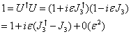
1 = [U dagger]U = ( 1 + i[epsilon][J₃ dagger]) ( 1 – i[epsilon]J₃)

= 1 + i[epsilon]([J₃ dagger] – J₃) + 0[epsilon]²

Now, you could either imagine this as keeping the axes fixed and rotating the physical system, or as keeping the physical system fixed and rotating the axes. A rotation of the physical system by θ is identical to a rotation of the axes by -θ. Therefore, the rotated wavefunction Ψ’ at the unrotated coordinate r is the same as the unrotated wavefunction Ψ at the rotated coordinate R^-1r.

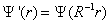
[psi]’ (r) = [psi] (R^-1 r)

Therefore, you have a one-to-one correspondence between Ψ’ and Ψ which we describe with the unitary representation.

[psi]’ = U[psi]

So now let’s look at an infinitesimal rotation about the z-axis. The z-coordinate is kept the same, while x and y are rotated by an infinitesimal rotation ε.

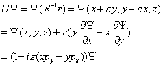
U [psi] (x, y, z) = [psi] (R^-1 r) = [psi](x + [epsilon]y, y + [epsilon]x, z)

= [psi](x, y, z) + [epsilon]( y[partial derivative of psi with respect to x] – x[partial derivative of psi with respect to y])

= (1 – i[epsilon](xp_y – yp_x))[psi]

Comparing with U = 1 – iεJ₃ you have

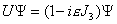
U[psi] = (1 – i[epsilon]J₃)[psi]

Therefore, we can identify the generator J₃ of rotations about the z-axis with the third component of the angular momentum operator.

The eigenvalues of the observable J₃ are constants of the motion. They are conserved quantum numbers. A symmetry of the system has led to a conservation law. The fact that experiments performed with different orientations of the apparatus give the same physics results has led to the conservation of angular momentum. This, of course, is the result of Noether’s Theorem, invented by Emmy Noether in 1915, which says that for every continuous symmetry of the laws of physics, there must exist a conservation law, and for every conservation law, there must exist a continuous symmetry.

A rotation through a finite angle θ may be built up from a succession of n infinitesimal rotations.

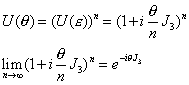
U([theta]) = U([epsilon])ⁿ = (1 + i([theta]/n) J₃)ⁿ

lim n -> infinity (1 + i([theta]/n) J₃)ⁿ = e^{-i[theta]J₃}

Now here we have done this whole thing for rotations around the z-axis, also called the 3-axis. You can do the same thing for the x-axis or 1-axis, to define J₁, as well as the y-axis or 2-axis, to define J₂.

You get the following results.

[ J₁, J₂ ] = iJ₃

[ J₂, J₃ ] = iJ₁

[ J₃, J₁ ] = iJ₂

You can write this compactly as

[ J_j, J_k ] = iJ_l

where jkl are cyclic permutations of 123. In fact, more generally you have

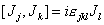
[ J_j, J_k ] = i[epsilon]_jklJ_l

where ε_jkl = +1 for a cyclic permutation of 123, -1 for an anticyclic permutation (321), and 0 otherwise. ε_jkl is called the structure constants of the group. The J’s form a lie algebra.

Non-linear functions of the generators which commute with all generators are called Casimir operators. For the rotation group, the only Casimir operator is J² = J₁² + J₂² + J₃²

This is in fact, the definition of a Lie group. The elements of a Lie group are

U([alpha]₁, [alpha]₂,…[alpha]_N) = e^{i[alpha]₁X₁ + i[alpha]₂X₂ +…i[alpha]_NX_N} = e^{i[alpha]_nX_n}

The N generators are Hermitian operators obeying a Lie algebra.

[X_a, X_b] = if_abcX_c

The generators form an N-dimensional vector space. Each generator is an operator in a Hilbert space parametrized by the angles α_a. The coefficients f_abc are the structure constants of the group.

There are many types of Lie groups. The following are the main ones.

Name	Algebra	Cartan Label	Number of Generators
Special Unitary	SU(n)	An-1	n2-1
Special Orthogonal	SO(n)	B(n-1)/2 if n odd Dn/2 if n even	(1/2)n (n-1)
Unitary Symplectic	Sp(n)	Cn/2	(1/2)n (n+1)

Then you have the exceptional groups, G₂, F₄, E₆, E₇, and E₈. There is an infinite series of simple Lie groups associated to rotations in real vector spaces which are the SO(n) groups, also called the B and D series. There is an infinite series of them associated to rotations in complex vector spaces which are the SU(n) groups, also called the A series. There is infinite series of them associated to rotations in quaternionic vector spaces which are the Sp(n) groups, also called the C series. The five exceptional groups are related to the octonions. The pure mathematics of Lie groups is excruciatingly complicated, and talks about things like nilpotent groups, etc. Here we’ll only discuss what’s used in particle physics. Most groups in particle physics are of the SU(n) type.

Elements of the SU(n) groups are represented by n x n unitary matrices. U^†U = 1 with det U = 1. Let’s determine the number of independent parameters. There are n x n = n² elements. Each is complex. Complex numbers, a + bi, each have two parameters so that’s 2n². U^†U = 1 imposes n conditions on the diagonal elements so that’s 2n² – n. From that you subtract the number of independent elements which is half those not including the diagonal. n x n = n² elements minus n diagonal elements is n² – n. You take half of those so that’s (n² – n)/2. You take twice that since they are complex 2[(n² – n)/2] = n² – n. Then subtract half those off the diagonal, n² – n, from the total minus the diagonal restrictions, 2n² – n.

(2n² – n) – (n² – n)

2n² – n – n² + n

2n² – n² = n²

Since det U = 1 is fixed, you end up with n² – 1 free parameters.

In particle physics, that is the number of bosons that mediate the force. The weak force is described by SU(2). 2² -1= 4 -1 = 3 bosons, which are the W⁺, W^–, and Z⁰. The strong force is described by SU(3), 3² – 1 = 9 – 1 = 8 bosons which are the 8 gluons. The minimal grand unified theory is SU(5). 5² – 1 = 25 – 1 = 24 bosons, which are the 12 bosons from the Standard Model, plus 12 new bosons which convert quarks to leptons and vice versa.

In the 2 x 2 case, the possible ways to parametrize U are

where a and b, which are called Cayley-Klein parameters, are complex numbers, and |a|² + |b|² = 1, or

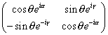
If H is Hermitian, meaning H commutes with H^†, then e^iH is unitary.

(e^iH)^†(e^iH) = e^-iH† e^iH = e^-i(H-H†) = e^-i(0) = 1

In a U(n) group, you have

U = e^iH

A subgroup of U(n) is the special unitary group SU(n). SU(n) has the further restriction that det U = 1

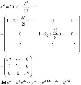
det U = det e^iH = e^{Tr H}

Tr H is the trace of the matrix H, which is the sum of the diagonal components. If the sum of the diagonal of H is 0, then H is called “traceless” and

det U = e^{Tr H} = e⁰ = 1

Here I show explicitly that det e^A = e^{Tr A}

In the lowest dimension non-trivial representation of the rotation group, j = ½, the generators can be written

J_i = (1/2) [sigma]_i where i = 1, 2, 3

where σ_i are the Pauli matrices

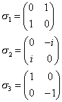
The basis for this representation is usually chosen to be the eigenvectors of σ₃ which are

The first describes a spin ½ particle of spin projection up along the z-axis.

m = + ½ or up

The second describes a spin ½ particle of spin projection down along the z-axis.

m = – ½ or down

The Pauli matrices σ_i are Hermitian, and the transformation matrices are unitary.

U([theta]_i) = e^{-[theta]_i[sigma]_i/2}

The set of all unitary 2 x 2 matrices is group U(2). The group of matrices U(θ_i) is smaller than this, and is represented by SU(2) which is a subset of U(2).

There are 1, 2, 3, 4, . dimensional representations of SU(2) corresponding to j = 0, ½, 1, 3/2, … respectively. The two-dimensional representation is the Pauli matrices themselves. They are called the fundamental representation of SU(2), the representation from which all other representations can be built.

The Pauli matrices have a simple generalization to SU(3). For SU(3), there are 3² – 1 = 8 generators. They are called λ_a where a = 1, 2, …8. The commutation relations are

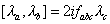
[ [lambda]_a [lambda]_b ] = 2if_abc[lambda]_c

where

f₁₂₃ = 1

f₄₅₈ = f₆₇₈ = 

f₁₄₇ = f₅₁₆ = f₂₄₆ = f₂₅₇ = f₃₄₅ = f₆₃₇ = ½

All other f’s are 0. f_abc is antisymmetric.

Here are the λ’s. They are also called the Gell-mann matrices. Compare to the Pauli matrices.

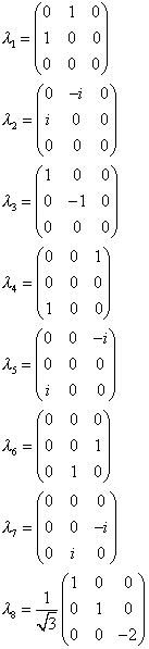
λ₃ and λ₈ are the only ones that are diagonal. σ₃ is the only one of the Pauli matrices that is diagonal. The number of Casimir operators is equal to the number of diagonal matrices.

A famous early experiment demonstrating the effects of quantum mechanics was the Stern-Gerlach experiment, performed by Otto Stern and Walther Gerlach in 1922. Let’s say you have a bunch of silver atoms in an oven, some of which escape through a small hole. The beam of silver atoms goes through a collimator, and then passes between two magnets, one of which has a sharp edge, so the beam is subjected to an inhomogeneous magnetic field. A silver atom has 47 electrons, 46 of which can be imagined to form a symmetrical cloud with no net angular momentum. Ignoring nuclear spin, the atom then has an angular momentum which is due solely to the intrinsic spin of the 47th electron, which is in the 5s orbital. The magnetic moment μ of the atom is proportional to the electron spin S. An atom with μ_z < 0, or S > 0, experiences a downward force. An atom with μ_z > 0, or S < 0, experiences an upward force. Therefore, the Stern-Gerlach experiment measures the z-component of μ, and thus the z-component of S. The atoms in the oven are randomly oriented. There is no preferred orientation of μ. If an electron were like a classically spinning ball, you would expect all values of μ_z to be realized between | μ | and -| μ |. You would then get one bundle of beams on the screen. Instead, however, the Stern-Gerlach experiment splits the original silver beam into two distinct components. This means that the electron spin S can only have two possible values of the z-component of S, which are spin up, S_z+, and spin down, S_z-. This shows that spin is quantized. In the same way, you could have split the beam into an S_x+ component and a S_x– component.

Now imagine that you do the Stern-Gerlach experiment, and divide the beam into S_z+ and S_z-. Now you let’s say you stop the S_z– beam, and using only the S_z+ beam, you do another Stern-Gerlach experiment, this time with the inhomogeneous magnetic field in the x-direction, and you divide the S_z+ beam into its S_x+ and S_x– components. According to classical physics, you would expect each of these beams not to contain any S_z– component since you already removed it. Now let’s say you stop the S_x– beam, and using only the S_x+ beam, do another Stern-Gerlach experiment, with the inhomogeneous magnetic field in the vertical direction. You might expect to only produce an S_z+ beam, but instead you produce both an S_z+ and S_z– beam. This shows that in quantum mechanics, you can’t measure both S_z and S_x simultaneously. The selection of the S_x+ beam erases any previous information about S_z.

You can represent the spin state of the silver atom, or actually the electron, in a two-dimensional abstract vector space. You can represent the S_x+ state by a vector called the ket, written as | S_x; + >, which is a linear combination of two base vectors, | S_z; + >, and | S_z; – >, which correspond to the S_z+ and S_z– states. Then you have

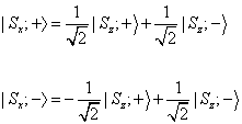
The 1/[squareroot of 2] factors are called Clebsch-Gordan coefficients.

If you have a function of a vector equal to a scalar times the vector, it takes the following form.

T(v) = [lambda]v

where T(ν) is the eigenfunction and is a linear operator, ν is the eigenvector, λ is the eigenscalar or eigenvalue, and λν is the eigenstate. “Eigen” is German for “his own” or “belonging to”. The terms eigenvalue and eigenvector probably originate from the idea that they are special values or vectors belonging to a matrix.

This is the notation that is used in quantum mechanics.

A | i> = a_i | i >

where A is the eigenfunction, and is an operator, | i > is the eigenvector, and a_i is the eigenscalar. ψ is the wavefunction and is a function of position. | ψ > is an operator.

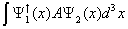
[integral] [psi]₁* (x) A [psi]₂ (x) d³x

can be written as

< 1 | A | 2>

A is an operator and can operate on 2, or its conjugate A^† can operate on 1. < 1 | is called the bra, and | 2 > is called the ket. Together, they form a bracket. Here you can read about bra-ket notation.

Kets are vectors in a complex vector space. Observables correspond to linear operators on that vector space. Physical states correspond to rays in this vector space, meaning that two kets represent the same physical state if and only if one ket is a complex number times the other ket. The 0 vector doesn’t correspond to a physical state. The counterpart of the ket space is called the bra space. It is a complex linear space, and there is a 1-1 mapping between a ket and a bra which is called the dual correspondence, represented by flipping the Dirac notation.

The Hermitian conjugate of an operator is

< [phi] | A | [psi] >* = < [psi] | A^† | [phi] >

If A = A^†, then A is a Hermitian operator.

If the eigenvalues are non-degenerate, the eigenfunctions are orthogonal, and can be defined to be orthonormal.

< i | j > = [delta]_ij

Such a set of eigenfunctions is called a complete set since any other state function can be expanded in terms of them.

Matrices have the same non-commutivity as operators and so can be used for the mathematical formalism of quantum mechanics. From matrix multiplication, where r is row, and c is column, you have

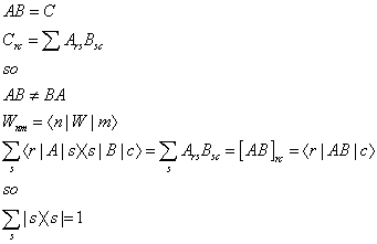
which is called the completeness relation.

In the early 20th century, quantum mechanics emerged with strange predictions: particles could be in superpositions, entangled with distant particles, and lack definite properties until measured. Many physicists hoped these oddities were just signs of an incomplete theory, that beneath quantum mechanics, a more “realistic” and “local” theory existed.

Locality means that objects are only influenced by their immediate surroundings, and that no information or effect can travel faster than the speed of light.

Realism holds that physical properties exist with well-defined values prior to and independent of measurement. In 1964, John Bell demonstrated that these assumptions, local realism, impose strict constraints on the outcomes of certain quantum experiments. These constraints are expressed as Bell Inequalities.

According to any local hidden variable theory (i.e., a theory that retains locality and realism), measurements on entangled particles must obey these inequalities.

But quantum mechanics predicts correlations that violate Bell inequalities. These correlations arise from entangled quantum states, where the measurement outcome of one particle is statistically linked to the other, even across vast distances.

Alain Aspect (1981 – 1982): Performed a series of experiments using entangled photon pairs. By switching measurement settings while photons were in flight, Aspect addressed the concern that information about the measurement setting might influence the source. His results clearly violated Bell inequalities.

Anton Zeilinger (1998): Pushed the boundaries by increasing the distance between entangled particles and improving detector efficiencies. This reduced the possibility of experimental loopholes, reinforcing that quantum mechanics predictions hold true.

Delft University (Netherlands): Used electron spins in diamonds and ensured space-like separation between measurement events.

NIST (USA): Used entangled photons with very high detector efficiency.

Vienna Group: Added randomness and fast switching to prevent signaling.

All these confirmed the violation of the Bell Inequalities while rigorously closing major loopholes:

1. the locality loophole (ensuring spatial separation) and

2. the detection loophole (ensuring all relevant outcomes are measured).

These results rule out any theory that preserves both locality and realism. At least one, or both, must be abandoned. If you keep locality, then you must accept nonrealism: the properties of particles are not determined until they are measured. If you keep realism, then you must accept non-locality: distant events can influence each other instantaneously. Some interpretations (like Bohmian mechanics) accept non-locality to preserve realism. Others (like Copenhagen) reject realism altogether. No consensus exists but the mathematical predictions of quantum theory are correct. Importantly, these violations do not imply that information travels faster than light. The correlations observed are strong, but do not allow controllable signaling, preserving consistency with special relativity. Bell’s Theorem is not just a test of quantum mechanics. It’s a test of how the world fundamentally works. It tells us that the Universe does not obey classical principles both locality and realism together.

There is a popular misunderstanding that consciousness is required for wavefunction collapse.

1. DOUBLE-SLIT EXPERIMENT BASICS :

When particles (like electrons or photons) pass through two slits without any measurement, they form an interference pattern—a wave-like behavior.

When which-path information is measured, the interference pattern disappears, and the particles behave like particles—suggesting “collapse” of the wave function.

2. QUANTUM ERASER VARIANTS :

In some experiments (like the quantum eraser), information about which-path the particle took is recorded but not accessed, or is scrambled.

In these setups, the interference pattern can reappear if the which-path info is truly unavailable, suggesting the availability of information affects the outcome. Some people misunderstand and think that consciousness causes collapse.

1. INFORMATION AVAILABILITY VS. CONSCIOUSNESS :

The experiments show that when which-path info is in principle unknowable, the system behaves like a wave. But this doesn’t mean a conscious mind must be involved. It suggests the physical availability of information, not an observer, is what matters.

2. NO-SIGNALING PRINCIPLE :

In quantum mechanics, information cannot be transmitted faster than light, and the outcome of a measurement does not depend on whether someone consciously observes it later. The idea that “consciousness collapses the wavefunction” has been proposed (e.g., by Wigner), but it is not experimentally proven.

3. ALTERNATIVE INTERPRETATIONS :

Decoherence explains wavefunction collapse as the system interacting with the environment, not any consciousness. Many-Worlds Interpretation says no collapse occurs, just branching realities. Objective Collapse Models like GRW add a spontaneous collapse mechanism.

It is not consciousness per se that causes wavefunction collapse, based on current evidence. Availability of information, not necessarily conscious observation, appears more relevant.

In the Schrodinger wave formalism, the time dependence is on the waves or states, and the operators are constant. In the Heisenberg matrix formalism, the time dependence is on the operators, and the waves or states are constant. In both cases, the time dependent part depends on the Hamiltonian. In the Dirac formalism, which is sort of a hybrid, both the waves or states, and the operators, are time dependent and depend on the Hamiltonian. The waves depend on the interaction Hamiltonian, and the operators depend on the free Hamiltonian.

Paul A. M. Dirac (1902 – 1984) attempted to combine special relativity with Schrodinger’s theory of wave mechanics. He took the following relation between kinetic energy and momentum.

E = (pv)/2 = (mv²)/2 = ((mv²)/2) (m/m) = (mv)²/2m = p²/2m

Einstein’s equation E = mc², and the mass of a particle as a function of rest mass

m = m₀/[squareroot of (1 – v²/c²)]

and used these to obtain the Klein-Gordon equation.

E² + p²c² = m₀²c⁴

Here the relationship between energy and momentum is symmetric because both are squared.

Erwin Schrodinger (1887 – 1961) derived the Klein-Gordon equation before inventing non-relativistic quantum mechanics. He actually used it to derive the fine structure constant of the hydrogen atom. However, he couldn’t get it to work because the Klein-Gordon equation does not fully describe fermions. Only after that did he turn to non-relativistic quantum mechanics, and wrote the Schrodinger equation. You take the de Broglie hypothesis.

P^u = i[h bar][partial derivative]^u

where

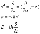
[partial derivative]^u = [partial derivative with respect to x_u] = ([partial derivative with respect to ct], –[nabla]) so p = -i[h bar] and E = i[h bar][partial derivative with respect to t]

and insert the substitutions into the energy-momentum relation E = p²/2m + V and you get

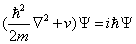
(([h bar]²/2m/)([nabla]^2/) + V)[psi] = i[h bar][psi]

Anyway, let’s go back to the Klein-Gordon equation derived by Dirac.

E² + p²c² = m₀²c⁴

If you solve for E, you get

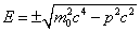
E = ± [squareroot of m₀²c⁴ – p²c²]

Now, the plus possibility means positive energy. The minus possibility means negative energy. Most people assumed that this negative solution was just a spurious result with no physical meaning. Dirac made the outlandish prediction that it refers to an actual particle that was an electron with negative energy. This particle was subsequently discovered by Carl Anderson in 1932 in a cloud chamber, and is called a positron.

In an atom, a photon can kick an electron from a lower to a higher level. Dirac imagined that there existed an infinite number of states below the lowest energy level in an atom, and they were all filled. A photon can kick an electron out of one of these states, and the positron is the hole left behind. When an electron falls into such a hole, a photon is released like an electron falling to a lower energy level in an atom. This was called the Dirac sea. We no longer imagine it like that, but we do imagine the vacuum as containing vacuum energy, and filled with particles continually coming in and out of existence. Dirac was the first to suggest a value for the vacuum energy, although his suggestion of negative infinity is obviously not accurate.

If you take Dirac’s version of the Klein-Gordon equation.

E = ± [squareroot of m₀²c⁴ – p²c²]

and make the normal operator substitutions we did earlier, you get

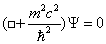
( [D’Alambert] + (mn²c²/[h bar]²))[psi] = 0

which is the normal way of writing the Klein-Gordon equation.

Dirac looked at his equation and thought that it must be possible to write it as a linear expression where the momentum p is a vector. He came up with

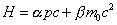
H = [alpha]pc + [beta]m₀c²

We saw before, the following notation.

[a, b] = ab – ba

This is called a commutator. The following defines an anticommutator.

{a, b} = ab + ba

If you insert the above Hamiltonian into the energy-momentum relation, then for self-consistency, α and β must obey the following relations.

[beta]² = 1

{[beta], [alpha]_i} = 0

{[alpha]_i, [alpha]_j = 2[delta]_ij

There are no numbers that obey these relations. Most people would say there was no solution, but Dirac thought there must exist some entities that would meet these criteria. He suggested that α and β were operators whose existence suggested a new degree of freedom.

Dirac found that such entities did exist, and they were a set of matrices that had been developed earlier by Wolfgang Pauli who used them to describe electrons as spin ½ particles, where one complete rotation is 720°.

α and β are 4 x 4 matrices.

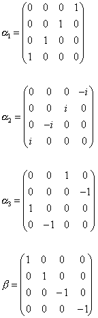
They are normally written down in Dirac representation.

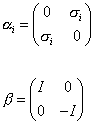
where σ_i are the three Pauli matrices.

and I is the 2 x 2 identity matrix.

A less common representation created by Hermann Weyl is the Weyl representation.

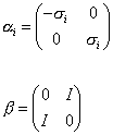
In these representations, the wavefunction is represented by a column vector called a spinor. It would be a digression to explain what exactly a spinor is but basically, it’s a thing that has to go through a rotation of 720° to return to its original state. This can be demonstrated by several parlor tricks.

Using α and β, you can define the gamma matrices as follows.

[gamma]⁰ = [beta]

[gamma]ⁱ = [beta][alpha]_i

They obey the following anticommutation relation.

{ [gamma]^u, [gamma]^v } = 2g^uv

Using the de Broglie operator

P_u = i[h bar][partial derivative]_u

The Dirac equation becomes

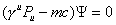
([gamma]^uP_u – mc)[psi] = 0

Sometimes you see the scalar product of a 4-vector with γ^u represented by a slash through the 4-vector.

[P slash] = [gamma]^uP_u

The gamma matrices can be written to form a 4-vector.

[gamma]^u = ([gamma]⁰, [gamma]^I

They obey the following relation.

[gamma]^u [gamma]^v + [gamma]^v [gamma]^u = 2g^uv

Another quantity you can define is γ⁵

[gamma]⁵ = i[gamma]⁰[gamma]¹[gamma]²[gamma]³

At one time, some people had the gamma indices run from 1 – 4, so the next one would be 5. However, most people run them from 0 – 3, so now there is no γ⁴.

We can define the chirality operator.

[Pi]^± = ½ (1 ±[gamma]⁵)

A state of definite chirality produces particles of one helicity in the massless limit. The weak interaction involves 1 – γ⁵ and thus produces only left-handed neutrinos.

In Dirac representation.

Another quantity you can define is the adjoint spinor [psi bar].

[psi bar] = [psi dagger] [gamma]⁰

The Hermitian conjugate denotes the complex conjugate of the transposed wavefunction. You take the vector transpose of the column vector ψ.

Using the following relations.

[gamma]^{0 dagger} = [gamma]⁰

[gamma]^{j dagger} = -[gamma]^j

j not equal to 0

you can write the Dirac equation in adjoint form.

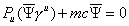
P_u ([psi bar] [gamma]^u) + mc[psi bar] = 0

Take the combination

[psi bar] [dirac] – [dirac bar][psi]

This gives

[partial derivative]_u ([psi bar] [gamma]^u [psi]) = 0

This suggests that

J^u = [psi bar] [gamma]^u [psi]

is to be interpreted as a probability 4-current.

You can call γ^u a 4-vector in the sense that [Ψ bar] γ^u Ψ, which is a scalar in spin space, transforms as a normal 4-vector, like p^u or x^u.

It’s sometimes useful to define the following operators which can isolate left-handed or right-handed particles of a given type.

The following interesting chronology describes how these developments came about.

1. Erwin Schrodinger takes the formula E² = p² + m² for kinetic energy in special relativity, replaces energy and momentum by operators, and gets a wave equation, which we now call the Klein-Gordon equation.

2. Schrodinger uses the Klein-Gordon equation to solve for the energy levels of the hydrogen atom. He gets answers he dislikes, so he never publishes this, and he discards the Klein-Gordon equation.

3. In 1926, Schrodinger tries again, starting from the formula E = p²/2m for kinetic energy in Newtonian mechanics. He gets answers he likes, publishes this work, and becomes famous. This equation becomes known as the Schrodinger equation.

4. In 1926, Oskar Klein and Walter Gordon, seeking to extend Schrodinger’s work to the relativistic case, reinvent the Klein-Gordon equation. It’s named after them since they published it first, even though Schrodinger derived it earlier.

5. People notice that the Klein-Gordon equation has negative-frequency solutions corresponding to the solutions of E² = p² + m² with E negative, and conclude something is wrong with the Klein-Gordon equation.

6. In 1928, Paul A. M. Dirac decides the Klein-Gordon equation has negative-frequency solutions because it’s a 2nd-order equation, and invents a first-order equation to replace it, called the Dirac equation.

7. Dirac discovers that the Dirac equation also has negative-frequency solutions, removing his initial motive for inventing it.

8. In 1929, Dirac interprets the negative-frequency solutions of his equation as negative-energy electrons, but uses the Pauli exclusion principle to argue that because electrons are fermions, this is okay as long as the negative-energy states are mostly filled. Dirac interprets the “holes” in the his negative-energy electron sea or Dirac sea to be positively charged particles with positive energy.

9. Since the only positively charged particles around are protons, Dirac argues that his holes are protons, even though his theory predicts they must have the same mass as the electron.

10. In 1931, Weyl convinces Dirac to come out and admit his theory predicts the existence of a new positively charged particle with the same mass as the electron, called the positron.

11. Researchers on cosmic rays notice that they had been seeing positrons for some time but ignoring them because everybody believed no such particle existed. The positron is now “discovered”, by Carl Anderson in 1932, meaning recognized.

12. Quantum field theorists realize that the Klein-Gordon equation is actually a correct description of spin-0 particles, and that for a complex-valued field the negative-frequency solutions correspond to antiparticles, just as in the Dirac equation. Since spin-0 particles are bosons, the Pauli exclusion principle does not apply here, so Dirac’s original argument involving “holes” cannot be used to explain why particles don’t sink into negative-energy states.

13. Quantum field theorists gradually straighten everything out, slowly dropping the “hole” story.

14. Condensed matter theorists studying semiconductors find that positively charged carriers are actually “holes” giving an example where Dirac’s idea is actually the best way to think about things. An electron and hole can form a bound state called an exciton.

There are three discrete symmetries that are commonly used in particle physics. Charge conjugation is when you replace every particle with its antiparticle. Parity inversion is if you hold up a mirror to the reaction, and look at its mirror image. Time reversal is if you run it backwards, analogous to filming it, and running the film backwards. This is how you would write down each of these symmetries.

C [psi] = [gamma]² [psi]*

P [psi] = [gamma]⁰ [psi]

T[psi] = [gamma]¹ [gamma]³ [psi]*

C, P, and T are symmetry operators. If a reaction is symmetric under these operations, then if you perform these operations, you still get a valid reaction.

The motivated reader can choose to derive the above equations. For charge conjugation, you take the wavefunction for a negative energy electron.

[psi] is proportional to e^{i(px + Et)/[h bar]}

and reverse the signs of p and E. Then swap ψ_U and ψ_D so that the negative energy states map onto part of the wavefunction that behaves correctly at low energies, and you also need a spin flip. It turns out that γ² will do that.

It used to be believed that all reactions obeyed C, P, and T symmetry. However, in 1956, it was proved that the weak force violated parity. It had previously been believed that parity was a conserved quantum number. Parity conservation was originally thought of by Eugene Wigner in 1927. According to this view, there were two particles, θ, which had even intrinsic parity, and τ, which had odd intrinsic parity.

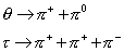
[theta] -> [pi]⁺ + [pi]⁰

[tau] -> [pi]⁺ + [pi]⁺ + [pi]^–

However, θ and τ had equal masses and lifetimes, and were identical in every way, so it seemed logical that they were one particle called K⁺, which meant parity is not conserved.

Remember

[gamma]⁵ = i[gamma]⁰[gamma]¹[gamma]²[gamma]³

This means that

[psi bar] [gamma]⁵ [psi]

is a psuedoscalar that reverses sign under coordinate inversion.

-[gamma]⁵ = [gamma]⁰ [gamma]⁵ [gamma]⁰

This means that parity will not be conserved. In October 1956, Lee and Yang suggested that parity was not conserved, and in December 1956, Wu and her team proved it using an experiment involving beta decay in cobalt-60. Chien Shiung Wu and her team worked with cobalt-60, which beta decays to nickel-60 with a half-life of 5.2 years. This is called a Gamow-Teller transition. The Co⁶⁰ nuclei had their spins aligned in a magnetic field. After the decay, the Ni⁶⁰ nuclei would have their spins aligned in the opposite sense, and this was checked by observing the spatial distribution of photons emitted in the subsequent gamma decays of Ni⁶⁰. Since the nuclear spin changes by one unit in the decay Co⁶⁰ → Ni⁶⁰ + e + [nu bar], then if L = 0, for the electron and antineutrino, their spins must point in the same direction to conserve angular momentum. If weak interactions conserved parity, half the time you would get a right-handed electron and left-handed antineutrino, and half the time, you would get a left-handed electron and right-handed antineutrino. Instead, you only get a left-handed electron, and right-handed antineutrino, which means that weak interactions do not conserve parity. It was realized that we only detect left-handed neutrinos and right-handed antineutrinos.

Then it was believed that all reactions obeyed C and P symmetry in combination, called CP, and also T. Then in 1963, it was realized from looking at kaon decay that CP symmetry was not always conserved. However, all reactions will obey CPT symmetry.

You can also discuss C, P, and T symmetry from the vantage point of group theory. A finite group is a group with a finite number of elements. One of the simplest groups has only two elements, the identity I, and an element g such that g² = e. Invariance under g is represented by the unitary operator.

[U, H] = 0

For a two element group, you have

U² = 1

since U is unitary, it is Hermitian. U is the observed quantity, and its eigenvalues are conserved quantum numbers.

U² | p> = p² | p>

where p is an eigenvalue of U corresponding to the eigenvector | p>. Since p² = 1, then the allowed eigenvalues of p are +1 and -1. Invariance of the system under symmetry operation g means that if the system is an eigenstate of U, then you can only go to states with the same eigenvalue. Here P and C are examples of the unitary operator U. Time reversal invariance requires an antiunitary operator.

{U, H} = 0

Throughout most of the 18th and 19th Century, the main focus of what to them was advanced physics was the study of electromagnetism. Scottish physicist James Clerk Maxwell (1831 – 1879) published his monumental work “A Dynamical Theory of the Electromagnetic Field” in 1864. He proved that the electric field and magnetic field were two aspects of one thing called an electromagnetic field. Today, this is so completely understood that no one in particle physics ever refers to such a thing as an electric or magnetic field. Today, these are recognized to be simply the two transverse polarized states of a photon, just as any massless particle has two transverse polarized states, and a massive particle also has a longitudinal polarized state.

The electromagnetic field is represented by A^μ which is related to the classical concepts of the electric and magnetic fields in the following way. You define the following antisymmetric tensor.

F^uv = [partial derivative]^u A^v – [partial derivative]^vA^u

where

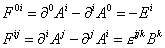
F⁰ⁱ = [partial derivative]⁰ Aⁱ – [partial derivative]ⁱA⁰ = -Eⁱ

F^ij = = [partial derivative]ⁱ A^j – [partial derivative]^jAⁱ = [epsilon]^ijkB^k

where E and B are the electric and magnetic fields. The Lagrangian for electromagnetism is

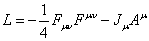
L = -(1/4) F_uv F^uv – J_uA^u

Electromagnetism has gauge freedom. It is not affected by adding a scalar field.

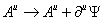
A^u -> A^u + [partial derivative]^u [psi]

where ψ is any scalar field, and has no effect. It does not alter the field tensor.

F^uv = [partial derivative]^u A^v – [partial derivative]^vA^u

Therefore, it is always possible to make a scalar field vanish.

For a massive particle, E = mc². In naturalized units, where c = 1, E = m. Therefore, mass and energy are interchangeable, and you are free to measure the mass of particles in units of energy. For photons, you are supposed to use the wave form, where E = [h bar]w, where w is the angular momentum. Also, p = [h bar]k where p is the momentum and k is the wave number. The wavenumber k = 2π/λ where λ is the wavelength. In naturalized units where [h bar] = 1, then E = w, and p = k, so for photons, energy and angular momentum are interchangeable, and momentum and wave number are interchangeable. In quantum field theory, you often see the following relation.

e^i(kx-wt)

This is called the plane wave, and is the wavefunction of a particle traveling in a straight line. If you do a Fourier expansion of an electromagnetic wave, you get two such things, with coefficients that are related to the annihilation and creation operators. These create and destroy particles, in this case photons, which relates the wave form to the particle form. This was first done by Max Born. You end up quantizing the field, which is why it’s called quantum field theory or second quantization.

Let’s say you have electromagnetic radiation in a box of volume V, where L is the length of a side, and V = L³. Now do a Fourier expansion.

A = 1/[squareroot of V] [summation of k, [alpha]] [c[epsilon]^(alpha)e^i(kx-wt) + c*[epsilon]^(alpha)e^-i(kx-wt)]

where the expansion coefficients c and c* are functions of the wavenumber k and α. α is an index labeling the polarization, which is described by two unit vectors, ε¹ and ε², which are perpendicular to k and to each other. The Hamiltonian of the system is

H = ½ [integral] (B² + E²)dV = ½[integral][([nabla] x A)² + [A dot]²]dV

You find that each half of the Hamiltonian gives the same result so that the total is

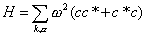
H = [summation of k, [alpha]] w² (cc* + c*c)

You can also take into account the possibility that the c’s depend on time by the redefinition

c(t) = ce^-iwt

Now let’s define the new variables.

q = c + c*

p = (w/i)(c – c*)

Then the Hamiltonian is

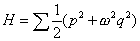
H = [summation](1/2) (p² + w²q²)

This is just the Hamiltonian of harmonic oscillations, which is what you would expect since the electric and magnetic fields are harmonic oscillators.

Now p and q are operators acting on a wavefunction, and obey the following commutation relation.

[q, p] = i[h bar]

Now let’s define the following ladder operator.

a = [squareroot of (2w/[h bar])]c

Then you end up with

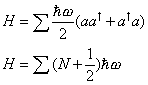
H = [summation]([h bar]w/2)(aa^† + a^†a)

H = [summation](N + (1/2))[h bar]w

where [a, a^†] = 1, and the number operator N = a^†a.

The number operator N = a^†a is Hermitian, and you have

N | n > = n | n >

You have the following commutators.

[a, N] = a

[a^†, N] = -a^†

a is the annihilation operator, and a^† is the creation operator.

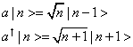
a | n > = [squareroot of n] | n – 1 >

a^† | n > = [squareroot of n + 1] | n + 1 >

Now look at the following equation.

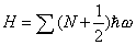
H = [summation](N + (1/2))[h bar]w

N is the number of particles, and see that even when N = 0, H is not zero. This is the origin of the idea that the vacuum itself has energy. The energy density of the vacuum is given by

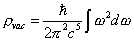
p_vac = ([h bar]/2[pi]²c⁵) [integral] w²dw

which, according to this, would be infinite. You can make it finite by assuming that this is a finite instead of infinite integral.

Now, you can think of the vacuum energy as caused by virtual photons, and if you have smaller and smaller waves of virtual photons going down to infinity, then that would be an infinite amount of energy. If there was some lattice that prevented such arbitrarily small waves, then the energy would be finite. That’s what you have inside a crystal in solid-state physics, and in that case, the equations predict what you observe. Now space itself could be quantized and form such a lattice but it would have to be at a smaller scale than we observe, since we don’t observe any such thing, and if that were true, the value of the vacuum energy, or zero point energy, would be 10¹²⁰ times higher than we currently observe. We currently have no explanation for this discrepancy. We can observe a small vacuum energy called the Casimir effect. If you have two parallel plates, only an integral number of standing waves of virtual photons can exist between the plates, while those on the outside have no such restriction. This causes a tiny force pushing the plates together, which has been experimentally detected. The Casimir effect was predicted by the Dutch physicist Hendrick Casimir in 1948, and was experimentally measured by Steven Lamoreaux in 1996.

I assume the reader has already read my other papers on tensors and Lagrangians. Even if you have already read them, you might want to look over my paper on Lagrangians to refresh your memory. The Lagrangian L is the kinetic minus potential energy. The integral of Ldt is the action S, and you choose the function x such that S will be stationary for small changes in x. For a more detailed account, read my paper on Lagrangians. This is the Lagrangian for an electromagnetic field.

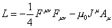
L = -(1/4) F^uv F_uv – [mu]₀J^uA_u

where

F^uv = [partial derivative]^u A^v – [partial derivative]^v A^u

This is the Lagrangian for a fermionic field

L = i[psi bar] [gamma]^u [partial derivative]_u [psi] – m[psi bar] [psi]

Now the really neat thing is all you have to do is add these two Lagrangians together to get the interaction between an electromagnetic and fermionic field.

L = L_f + L_em = = i[psi bar] [gamma]^u [partial derivative]_u [psi] – m[psi bar] [psi] – (1/4) F^uv F_uv – J^uA_u

Here the 4-current J^u is the quantum 4-current from the fermionic field, which is charge times the probability 4-current.

J^u = e [psi bar] [gamma]^u [psi]

This is the interaction term. It describes the mixing of the two fields. If you think of fields as sums of creation and annihilation operators, then these mixed terms allow you to change the number of two species simultaneously. This resulting theory is called quantum electrodynamics or QED.

To use the QED Lagrangian to calculate things, you need the perturbation to the Hamiltonian. If you make a perturbation to the Lagrangian, L → L + ΔL, since

H = p[q dot] – L

the perturbation to the Hamiltonian is ΔH = -ΔL so

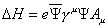
[delta]H = e [psi bar] [gamma]^u [psi] A_u

If I were to approach quantum field theory rigorously, I would first discuss φ⁴ theory, which is the simplest quantum field theory, having only scalar fields. The two-point correlation function or two-point Green’s function is <Ω|Tφ(x)φ(y)|Ω>, where |Ω> is the ground state of the interacting theory, which is different from |0> which is the ground state of the free theory. T is the time-ordering symbol. The correlation function can be interpreted as the amplitude for the propagation of a particle or excitation from y to x. If you have <0|Tφ{(x₁)φ(x₂)…φ(x_n)}|0>, which is the vacuum expectation value of time-ordered products of a finite number of free field operators, you can greatly simplify the calculations, which involves putting them in all possible combinations, by using Wick’s Theorem. From this, you can determine all possible Feynman diagrams of an interaction.

In particle physics, you often describe scattering events, where particles enter from infinity, interact, and then fly off. The transition between different states can be described by the following operator.

[psi] (t) = U(t, t₀) [psi] (t₀)

where the transition operator is the S-matrix.

U([infinity], -[infinity]) = S

The U operator satisfies the Schrodinger equation which is integrated to yield the following equation.

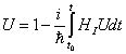
U = 1 – (i/[h bar]) [integral to t₀ to t] H_I Udt

where H_I is the interaction term of the Hamiltonian. H = H₀ + H_I The U matrix is unitary. U^-1 = U^†

As you see, U appears in its own definition, so you can’t solve for S exactly but it can only be solved iteratively by continually plugging in the results to get a better approximation.

S = 1 – i[integral]H_Idt + (-i)²[integral]H_I(t₁)dt + [integral from -infinity to t₁]H_I(t₂)dt + …

A version of the S-matrix called the bootstrap method at one time was an alternative to the theory of quarks, and gave rise to Regge theory. The theory of quarks and the Standard Model won that argument. However, Regge theory helped inspire early string theory, which is now our way of viewing the Universe.

The interaction Lagrangian is a mixture of creation and annihilation operators. For quantum electrodynamics, you have

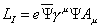
L_I = e [psi bar] [gamma]^u [psi] A_u

The successive higher orders of perturbation theory represent the creation and annihilation of more and more particles as part of the intermediate stage of the scattering process.

An easy way to write down a given scattering process, and the creation and annihilation of particles, is by Feynman diagrams. The interaction Hamiltonian for QED describes the creation and annihilation of electrons, positrons, and photons. There are eight possible combinations which are drawn below. Here I’ve drawn t as the horizontal axis, and x as the vertical axis, although sometimes it’s shown reversed. Arrows pointing towards increasing time are electrons, arrows pointing backwards are positrons, and wavy lines are photons.

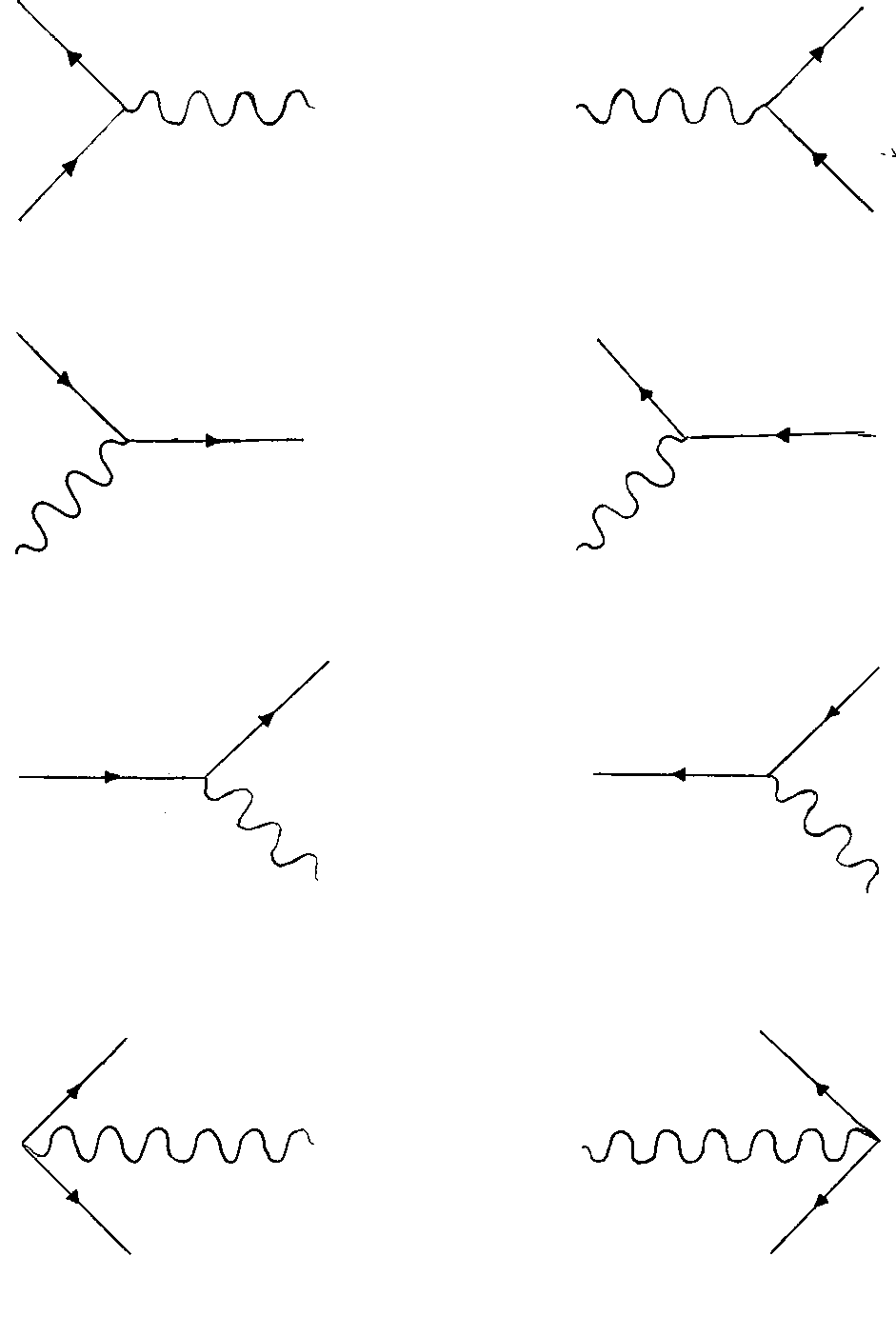
Now, your gut feeling is to imagine these as pictures of physical particles flying through space, interacting, and flying off. That’s not really what it is. Remember that in quantum mechanics, what really exists when you’re not measuring it is the wavefunction, which can be identified with the probability of detecting a particle. Here, the creation and annihilation operators describe the excitation of plane wave states rather than particles. The spacetime coordinates are variables to be integrated over rather than the positions of particles. Really, these diagrams are a non-algebraic representation of the S-matrix element.

None of these eight diagrams are possible all by themselves since they violate conservation of energy-momentum. You need two diagrams together so the failure of energy-momentum conservation in one diagram is cancelled out by that of the second.

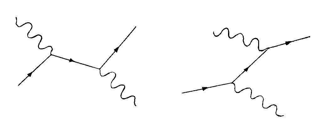
Compton scattering is e^– γ → e^– γ. Moller scattering is e^– e^– → e^– e^–. Bhabha scattering is e⁺ e^– → e⁺ e^–. Rutherford scattering is the scattering of an electron by a proton or neutron. Electron-positron annihilation is e⁺ e^– → 2γ.

Here are some examples of such processes. Here is Compton scattering, where there is an electron and photon in both the initial and final states.

Here is the diagram for Moller scattering where there is two electrons in both the initial and final states.

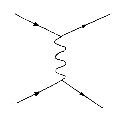
A Feynman diagram has external lines, which are particles that either enter from or exit to infinity, and internal lines, which are particles that exist only inside of the reaction. These internal particles are called virtual particles. You see that in Moller scattering, the two electrons exchange a virtual photon. Electromagnetism is nothing more than the exchange of virtual photons between charged particles. The other forces are also nothing more than the exchange of virtual bosons between particles. The strong force acts by the exchange of virtual gluons. The weak force acts by the exchange of virtual W⁺, W^–, and Z⁰ bosons. Gravity acts by the exchange of virtual gravitons.

Virtual particles do not obey the same rules as normal particles. The energy and momentum of normal particles obey the mass shell condition.

P^u P_u = m²

This is not true for virtual particles. Unlike a normal photon, a virtual photon will not satisfy E = pc.

However, many popular accounts of virtual particles are inaccurate. It is often said that virtual particles are created by borrowing energy. Actually, energy is conserved at the vertex. Also, in many books, it says that virtual particles can only be exchanged over subatomic distances. Actually, virtual photons are massless, and thus of infinite range. This should hardly be surprising since otherwise electromagnetism would not be a long range force. If a compass needle points north, that means that virtual photons are traveling tens of thousands of miles from the tip of the compass needle to the magnetic north pole of the Earth. If Earth orbits the Sun, instead of flying off at a tangent, that means it’s gravitationally bound to the Sun, which means that virtual gravitons are traveling 93 million miles between the Earth and the Sun.

One explanation of this is based on the Uncertainty Principle derived by Werner Heisenberg in 1927, where

[delta]x [delta] p > [h bar]

where Δx is the uncertainty in position, and Δp is the uncertainty in momentum. According to this, creation of a massless particle such as a photon requires a tiny amount of energy and momentum. Thus Δp is very small, and Δx is very large, which causes it to be a long range force.

The beauty of Feynman diagrams is that it allowed you to quickly write down any interaction algebraically, and solve scattering problems. Before Feynman diagrams, only an elite group of specialists worked with these sort of problems. Feynman diagrams opened up QED to the masses, comparatively speaking, in that any physicist could now do these problems. You define a covariant scattering matrix M_f that factors out the general features of the problem from the S-matrix.

S_fi = [delta]_fi + (2[pi])⁴ [delta]⁽⁴⁾ (P^u_in – P^u_out) [squareroot of F(E)] M_fi

where P^u is the 4-momentum summed over all particles, and the function F(E) accounts for all normalization constants in the field expansion.

F(e) = [pi]_in (2VE)^-1 [pi]_out (2VE)^-1 [pi]_f (2w)

where the last term is for fermions.

Feynman realized you could write down the invariant amplitude M just by looking at the diagram. The various factors are multiplied together, and integrated over the 4-momenta of the internal lines.

M = (2[pi])^-4 [integral] _____d⁴q

In the blank, you multiply together the terms from the Feynman rules.

1. For each vertex, write ie[gamma]^[alpha]

2. For each internal photon line of 4-momentum k, write (-ig_{[alpha][beta]})/k² + i[epsilon])

3. For each internal fermion line of 4-momentum p, write i/([p slash]- m + i[epsilon])

4. For each external input electron, write u_r(p)

5. For each external output electron, write [u bar]_r(p)

6. For each external input positron, write [v bar]_r(p)

7. For each external output positron, write v_r(p)

8. For each external input or output photon write [epsilon]_r[alpha](k)

9. For each closed fermion loop, multiply by -1, and take the trace over spinor indices, meaning summing over spin states of the virtual electron-positron pair.

Up till now, we have only considered the first terms in the S-matrix which give rise to tree level diagrams without loops. Here is the first order approximation for Moller scattering, where two electrons exchange a photon.

However, this is not the only possible diagram that could explain this reaction. Here are two second order diagrams.

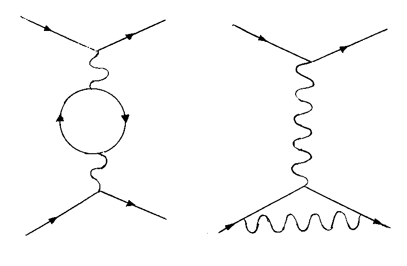
Indeed, there are an infinite number of possible diagrams. In order to truly calculate cross sections or anything else about these or any other particle interactions you would have to sum the results from an infinite number of Feynman diagrams, which is clearly impossible. However, this is not as serious a problem as it would first appear. Notice that the first order diagram has two electron-electron-photon vertices, while the second order ones have four each. For each such vertex, you multiply by e. In general, for n photons, you multiply by e²ⁿ. Therefore, each term in the perturbation series is about e² = 1/137 times smaller than the one before it. Therefore, you can just look at the first order approximation, or at most second order, and have a very good approximation.

In 1947, Lamb and Rutherford found that the s state of the hydrogen atom had slightly higher energy than what was predicted by quantum mechanics. This is called the Lamb shift, and is explained if you include the one loop corrections in the Feynman diagrams.

However, there is a deeper problem with QED than this. Let’s look at this diagram.

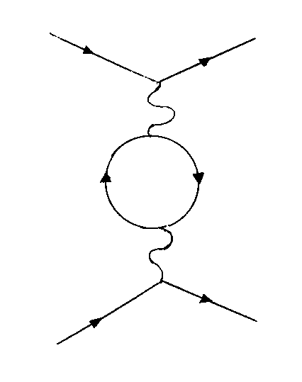
Due to the conservation of energy-momentum, the momentum of the photon is divided between the electron and positron on the internal loop. There are an infinite number of ways it can be divided between them, and you have to take them all into account. You have to sum over the infinite range of momenta of the two particles. You can perform integrals over the infinite range of loop momenta, but when you do that, the integrals diverge.

The solution to this problem is called renormalization, and was developed in the late 1940’s by Sin-Itiro Tomonga, Julian Schwinger, and Richard Feynman, who shared the 1965 Nobel Prize for their work. An example of renormalization is that an electron is surrounded by a cloud of electron-positron pairs that partially cancel its electric charge. Thus as you get closer to an electron, you partially penetrate this cloud, and its measured value of its electric charge increases. You could say its bare charge is infinite, and there is an infinite number of electron-positron pairs, so their effect is also infinite. These two infinities cancel each other out, leaving the measured value of an electron’s charge from a distance. Essentially two values which you have no way of knowing, and are in some sense mathematically infinite, combine to give a value you can measure. In this way, infinities are absorbed into physical constants, and QED is made to work. Another example is the electron’s measured mass which is the bare mass plus the self-energy which is the result of the electron continually admitting and reabsorbing photons.

The problems associated with renormalization are related to the vacuum energy. A theory that produces infinities when no particles at all are present, can hardly be expected to behave better in a more complicated situation. Despite these difficulties, renormalization is more easily dealt with in QED than anywhere else in particle physics.

You can think of renormalization the following way. You only calculate the theory to a certain energy or distance called the cut-off. As you let the cut-off distance go to zero, the predicted bare values of various quantities change and might go to infinity, which is fine since it’s assumed that quantum effects which we don’t know about will combine with the bare values to create the measured values we know about. You might have quantities whose measured value is zero change to non-zero. You just have to make sure you have enough parameters to begin with. If you only need a finite number of parameters, it works out, and the theory is renormalizable. If you need to add a infinite number of parameters, it does not work, and the theory is nonrenormalizable. Another thing you can do is the renormalization group or regularization. Here you are changing not the cut-off distance but the distance at which you are making the measurements, and letting that go to infinity. Often, nonrenormalizable terms in the theory will go to zero at long distances. Therefore theories that we use all the time, and work fine, might break down at very high energies or small distances, but we don’t have to worry about that, because they work fine at the energy scales at which we use the theory. In some interpretations of string theory, there are not four but an infinite number of forces, but all but four are negligible at less than the highest energies, and so we don’t know about them.

Richard Feynman also came up with a path integral formalism where the integral kernel, or propagator, of the time evolution operator can be expressed as a sum over all possible paths between two points.

The Standard Model rests on the assumption of gauge symmetry. This is where if you do a transformation, it doesn’t affect the validity of the results. A gauge symmetry indicates a hidden degree of freedom. In electromagnetism, you can make the following transformation.

A -> A + [nabla]X

In quantum mechanics, the Lagrangians describing a quantum field will be invariant under the transformation.

[psi] -> [psi]e^i[theta]

where θ is any constant angle. This is called global gauge symmetry. However, in quantum theory, the phase should be locally unobservable, meaning hidden. Therefore, it should be invariant under the following local gauge transformation.

[psi] -> [psi]e^i[theta]xu

However, the Lagrangians do not initially appear to be invariant under this transformation.

Let’s say you have the Dirac Lagrangian.

L = i[psi bar][gamma]^u [partial derivative]_u [psi] – m² [psi bar] [psi]

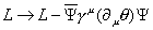
Under the local transformation, it will transform as

L -> L – [psi bar] [gamma]^u ([partial derivative]_u [theta]) [psi]

The gauge transformation will have observable consequences. The problem is you have terms with the derivative of θ. You want to get rid of them the same way you could if θ was a constant. The way around this is to add a term whose purpose is to cancel out the unwanted θ terms. You replace ∂^u with ∂^u + V^u

[partial derivative]^u with [partial derivative]^u + V^u

Then you make the transformations.

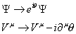
[psi] -> e^i[theta] [psi]

V^u -> V^u – i[partial derivative]^u [theta]

Then the terms cancel, and you have local gauge invariance. However, in order to do this, you have to add a new field V^u. You don’t want this new field to spoil the gauge invariance, so its derivatives must occur in the antisymmetric combination.

F^uv = [partial derivative]^uV^v – [partial derivative]^vV^u

so the simplest kinetic energy term is F^uvF_uv.

Thus the resulting Lagrangian for a fermion field is

L = I[psi bar] [gamma]^u D_u [psi] – m² [psi bar] [psi] – (1/4)F^uvF_uv

where

D_u = [partial derivative]_u + ieA_u

The new field is essentially the QED Lagrangian. Notice how this resulted automatically from making the Dirac equation locally invariant. The field we invented just to cancel unwanted terms turned out to be electromagnetism. This is what you have throughout the Standard Model. With the other forces, you introduce a vector field to get rid of the 4-vector ∂^u. This creates new terms in the Lagrangian that are to be identified with the particle that mediates the interaction. Because they are vector fields, the particles are spin-1 gauge bosons. They arise automatically as a result of making the Lagrangian locally invariant.

In the 1920’s, physicists had a semi-classical view of the atom, based on analogy with the Solar System. In the Solar System, the planets orbit the Sun, and also rotate on their axes. Similarly, in the Bohr model, the electrons were imagined to orbit the nucleus, and also spin on an internal axis like a top. However, since this was semi-classical, only certain values were allowed. Angular momentum about the nucleus was quantized in integer multiples of [h bar], and angular momentum about their axis, or spin, was quantized in half-integer multiples of [h bar]. Angular momentum, L, and spin, S, were two of the quantum numbers that identified an electron in an atom, the third being what electron shell it’s in. Setting [h bar] = 1, the spin of an electron could be either + ½, 0, or – ½. The intrinsic spin of a particle is the absolute value of its maximum, so an electron has a spin of ½. Particles with integer spin are called bosons. Particles with half-integer spin are called fermions. Fermions obey the Pauli Exclusion Principle, while bosons do not. The reason is because fermions have antisymmetric wavefunctions which cancel out when there’s more than one, while bosons have symmetric wavefunctions.

An electron has to rotate 720° to return to the same state. Most people assume this has something to do with the weirdness of quantum mechanics but actually that’s not true. There is an entirely classical type of spin where something has to rotate 720° in order to return to its original state, and this is described mathematically by a spinor. This can be demonstrated by several parlor tricks, such as Dirac’s scissors, Dirac’s belt, Dirac’s candle, Dirac’s teacup, etc. The spin of a particle is also described by the same mathematical entity.

It should be emphasized that the Solar System model was abandoned in the 1930’s. Names such as spin and angular momentum in particle physics are now considered metaphorical and have nothing to do with the classical meanings of the words. In particle physics, an electron is considered a zero-dimensional entity with zero volume so it’s meaningless to talk about it rotating in any literal sense. Spin is simply one of several quantum numbers that identify particles, and how they interact with other particles, and have nothing to do with any measurable characteristics of macroscopic objects. Julian Schwinger said, “For fundamental properties, we will borrow only names from classical physics”.

Spin is described by an SU(2) symmetry. SU(2) is a non-Abelian symmetry. The idea of non-Abelian gauge theories was first suggested by Chen Ning Yang and Robert Mills in 1954. Such theories are called Yang-Mills theories. In 1971 – 1972, Gerard ‘t Hooft, and Martinus Veltman came up with a renormalizable version of Yang-Mills, for which they received the 1999 Nobel Prize in physics. You can graphically represent spin in the following way. You could imagine drawing a vector in spin space, where it either points up or points down. Thus the two states are spin up or spin down. These are considered two states of one particle.

Then people thought up the idea that you could have a symmetry analogous to spin called isospin, where the two states of a particle are not spin up and spin down, but the proton and neutron. This might seem unusual, but from the point of view of particle physics, the proton and neutron are almost identical. Look at the masses of the proton and neutron.

proton – 938.28 MeV

neutron – 939.57 MeV

Their masses differ by only 0.1%.

The proton has electric charge of +1, and the neutron has electric charge of 0. However, electromagnetism is only 1% as strong as the strong force. Due to these slight differences, the SU(2) symmetry is not exact but it’s close.

Isospin is also described by an SU(2) symmetry. You can imagine drawing a vector in isospin space, and if it points up, it’s a proton, and if it points down, it’s a neutron. These are considered two states of a single particle called a nucleon. It’s mathematically the same as spin in that the isospin generators satisfy

[I_j, I_k] = i[epsilon]_jklI_l

In the fundamental representation, the generators are denoted I_i = (½ )τ_i where

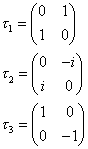
are the Pauli spin matrices. They act on the proton and neutron states.

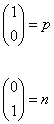
The nucleon then forms a doublet.

Other hadrons can also be classified as states in SU(2) multiplets. The less similar the particles, the less the symmetry will hold. The pions are placed in the following states.

where

[pi]^± = (-[pi]₁ Â± I[pi]₂)/[squareroot of 2]

[pi]⁰ = [pi]₃

Therefore, you can talk about the isospin of other particles. In general, the most positively charged particle is chosen to have the maximum value of the third component of isospin I₃.

In the early study of hadrons, the following formula was used to relate electric charge to isospin.

Q = I₃ + B/2

where Q is electric charge, B is baryon number, and I₃ is the third component of isospin.

Later, a class of particles was detected in the high-energy regime typical of strong force interactions, but whose lifetimes were relatively long, typical of the weak force. This was considered strange behavior, and so they were called strange particles. In 1953, Murray Gell-Mann invented a new quantum number called strangeness.

The equation was then modified.

Q = I₃ + (B + S)/2

where S is strangeness. This is called the Gell-Mann-Nishijima formula. Baryon number plus strangeness is called hypercharge.

Y = B + S

Q = I₃ + Y/2

The spin states up and down gave their names to the isospin states up and down, which in turn gave their names to the up and down quarks. The proton is two up quarks and a down quark. The neutron is two down quarks and an up quark. Strangeness was also identified with a quark called the strange quark.

According to the Standard Model, there are three generations of particles, each containing two quarks, and two leptons, one of which is a neutrino. In the first generation, there is the up and down quarks, the electron, and electron neutrino. In the second generation, there is the strange and charm quarks, the muon, and the muon neutrino. In the third generation, there is the bottom and top quarks, the tau, and the tau neutrino. These are all fermions. In addition, there are the bosons that mediate the forces. The photon mediates electromagnetism. The eight gluons mediate the strong force. The W⁺, W^–, and Z⁰ mediate the weak force. The Standard Model does not include gravitation, but gravity is mediated by the graviton. Also, according to the Higgs mechanism, which I describe later, there is a scalar particle left over called the Higgs particle.

Here are the fundamental particles.

Name	Mass	Charge	Color	Spin	Baryon Number	Lepton Number	Year First Detected
up quark	6 MeV	2/3	R, B, G	1/2	1/3	0	1967
down quark	10 MeV	-1/3	R, B, G	1/2	1/3	0	1967
strange quark	0.25 GeV	-1/3	R, B, G	1/2	1/3	0	1967
charm quark	1.2 GeV	2/3	R, B, G	1/2	1/3	0	1974
bottom quark	4.3 GeV	-1/3	R, B, G	1/2	1/3	0	1977
top quark	175.6 GeV	2/3	R, B, G	1/2	1/3	0	1995
electron	0.511 MeV	-1	none	1/2	0	1	1897
electron neutrino	0.05 eV < m < 0.45 eV	0	none	1/2	0	1	1953
muon	0.106 MeV	-1	none	1/2	0	1	1937
muon neutrino	< 0.17 MeV	0	none	1/2	0	1	1962
tau	1.777 GeV	-1	none	1/2	0	1	1975
tau neutrino	< 24 MeV	0	none	1/2	0	1	2000
photon	0	0	none	1	0	0	wave – 1690 particle – 1905
W+, W–	80.3 GeV	+1, -1	none	1	0	0	1983
Z0	91.2 GeV	0	none	1	0	0	1983
gluon	0	0	, , , , , , ,	1	0	0	1979
graviton	0	0	none	2	0	0	not yet
Higgs particle	125.3 ± 0.6 GeV	0	none	0	0	0	2012

In the above list, the strange quark has a strangeness of -1, and all other particles have a strangeness of 0. Antiparticles have opposite signs for electric charge, baryon number, and lepton number, and have anticolors instead of colors. Colored particles only exist in combinations in which the colors cancel out. Baryons are three quarks. Antibaryons are three antiquarks. Mesons are quark-antiquark pairs. Glueballs are gluon-antigluon pairs. Baryons, antibaryons, and mesons are hadrons. A tetraquark is two quarks and two antiquarks. A pentaquark is four quarks and an antiquark.

For the photon, I have given the years that Christiaan Huygens proposed the wave model, and Albert Einstein proposed the particle model to explain the photoelectric effect, instead of year of first detection, since of course you are detecting photons with your eyes whenever you see. Newton had also believed that the photon was a particle. For the electron neutrino mass, I am using the results from the Karlsruhe Tritium Neutrino (KATRIN) experiment from April 2025. The discovery of the Higgs boson, the last particle of the Standard Model to be detected, was announced by the ATLAS and CMS collaborations at the Large Hadron Collider (LHC) at CERN on July 4, 2012. We will never be able to detect gravitons directly because they are so weakly interacting but gravitons are the quantization of gravitational waves in the same way that photons are the quantization of electromagnetic waves. While Einstein proposed the existence of gravitational waves in 1916, their direct detection wasn’t achieved until 2015 by the Laser Interferometer Gravitational-Wave Observatory (LIGO).

Here are the relative strengths of the four forces.

strong – 10

electromagnetic – 10^-2

weak – 10^-5

gravity – 10^-40

In the beginning of the 20th Century, atoms were imagined to have positive and negative charges spread uniformly throughout. Then in 1909, Ernest Rutherford’s team fired alpha particles, which are helium nuclei, at aluminum foil, and some were bounced back, meaning that most of the mass of the atom was in a small dense core. In 1919, Rutherford proved that by bombarding air with alpha particles, a particle could be dislodged from the nitrogen nucleus. This particle appeared identical to the hydrogen ion. This suggested that atomic nuclei were made of these particles, which we now call protons. However, the proton has a positive charge, and a bunch of them are tightly packed in the nucleus. Electric repulsion should cause the nucleus to fly apart. Evidently, the electromagnetic force between them was compensated by a new mysterious force that attracted protons to each other. Since it was stronger than the electromagnetic force, it was called the strong force.

In 1935, Japanese physicist Hideki Yukawa predicted that there must exist some particle that mediated the strong force, analogous to the photon. The first hadron other than the nucleons to be discovered was the pion in 1947, and this was identified with Yukawa’s strong force carrier. However, this was only the beginning, as a very large multitude of new particles were then discovered, first in cosmic rays, and then in accelerators. Independently, Murray Gell-Mann and George Zweig arranged these particles in patterns based on their properties, which could be explained by the idea that they were composed of smaller constituents. Gell-Mann named these hypothetical constituents “quarks” after a line in James Joyce’s “Finnegan’s Wake” that read “three quarks for Muster Mark”. The constituent quark model was remarkably successful in predicting new particles, and explaining their characteristics.

Despite the phenomenological success of the constituent quark model, there was one obvious flaw in that no quark had ever been detected. Searches for the tell-tale fractional charge came up null. People even searched for quarks in mud and seawater. Many people were of the opinion that quarks were a useful computational tool but did not actually exist. Then in 1967, Jerome Friedman, Henry Kendall, and Richard Taylor at SLAC bombarded protons with electrons. In these inelastic collisions, they detected point-like constituents inside the proton, which were later identified with quarks. However, still no one had managed to observe a free quark outside a hadron. There was one baryon, the Δ⁺⁺, which in the quark model was supposed to be composed of three up quarks, all spin up. They would all have to have the same quantum numbers which would violate the Pauli Exclusion Principle, which states that more than one fermion can’t occupy the same state. Therefore, they invented a new quantum number which could be different for the three quarks, so they wouldn’t all be the same. Later, this property was called color, and was used to explain why you never see free quarks.

The word “color” comes from color theory where red, blue, and green combine to form white. Here quarks only combine in combinations that are colorless.

baryon – red, blue, green

antibaryon – antired, antiblue, antigreen

meson – red-antired, or blue-antiblue, or green-antigreen

Quarks are red, blue, or green. Antiquarks are antired, antiblue, or antigreen. In some old books, they use the following terminology.

antired = cyan

antiblue = yellow

antigreen = magenta

Here are the wavefunctions of the baryon and meson.

Baryon-

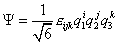
[psi] =(1/[squareroot of 6]) [epsilon]_ijkq₁ⁱ q₂^j q₃^k

Meson-

[psi] = (1/[squareroot of 2]) q₁ⁱq₂^-i

Originally, Murray Gell-Mann and others put the up, down, and strange quarks in an SU(3) invariant theory.

However, this was only an approximate symmetry. Later, it was realized that the more fundamental SU(3) symmetry was an exact one based on colors.

where the strong force Lagrangian is

L = [summation]_flavors [psi bar] (i[gamma]^u D_u + m) – (1/2)Tr F_uvF^uv

This is called quantum chromodynamics or QCD.

The covariant derivative is a 3 x 3 matrix.

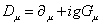
D_u = [partial derivative]_u + igG_u

where G_u is a combination of vector gauge fields called gluons and the generators Λⁱ

G_u = (1/2)G_uⁱ/\ⁱ

The gauge invariant field tensor is given by

F_uv = [D_u, D_v]/ig = [partial derivative]_uG_v – [partial derivative]_vG_u + ig[G_u, G_v]

The QCD Lagrangian can be written as

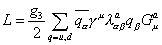
L = (g₃/2) [summation]_{q = u, d} [q bar]_[alpha] [gamma]^u [lambda]^a_{[alpha][beta]} q_[beta] G_u^a

where g₃ is the strong force coupling constant, and G_u^a is the gluon field.

Now there is a big difference between QED and QCD. If you look at the Pauli matrices, they are diagonal but if you look at the λ Gell-Mann matrices, they are not all diagonal. Therefore, the photon does not possess electric charge but the gluons do possess color charge. This means that the color of a quark can be changed by exchanging a gluon.

Each gluon has a color and anticolor. This would give nine combinations. However, due to SU(3) symmetry, the colors combine to form the states that are actually realized. They are arranged into a octet and singlet analogous to what I’ll show later for the up, down, strange SU(3) group. The SU(3) color octet forms the gluon colors which are as follows.

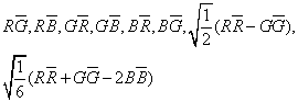
R[G bar], R[B bar], G[R bar], G[B bar], B[R bar], B[G bar], [squareroot of ½](R[R bar] – G[G bar]), [squareroot of 1/6](R[R bar] + G[G bar] – 2B[B bar])

The last two don’t change the colors of the quarks that exchange them. The color singlet does not carry color, and can’t mediate between color charges. Here is the SU(3) color singlet. It is associated with the meson state. It would be more accurate to say that this is the color of a meson since it is invariant under rotations in color space.

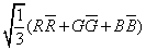
[squareroot of 1/3](R[R bar] + G[G bar] + B[B bar]

This color singlet state is also believed to refer to a particle called a pomeron, which is a colorless particle, whose exchange in an event is indicated by a rapidity gap, which is a region without particles. The virtual pomeron, which is presumed to be exchanged in diffractive processes, appears as a color singlet construct of quarks and gluons, perhaps a glueball.

Let’s compare Feynman diagrams for electromagnetism and the strong force. On the left is two electrons exchanging a photon. On the right is two quarks exchanging a gluon.

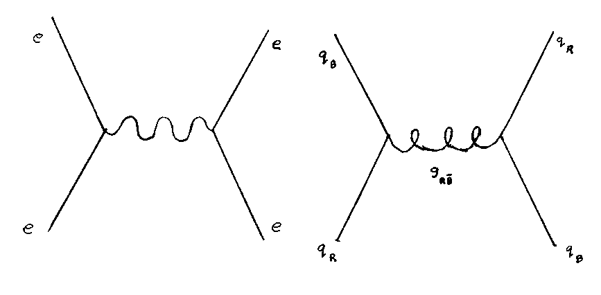
Now, the photon has no electric charge, and so the electrons might change momentum but their charges are not affected. The gluon, however, can carry color charge away from or to a quark. Here the gluon is red-antiblue. When a red quark emits a red-antiblue gluon, the quark changes from red to blue. When a blue quark absorbs a red-antiblue gluon, the blue quark turns red. You can draw the reaction like this.

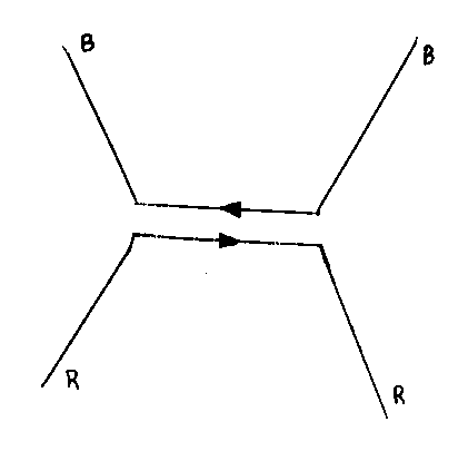
Here you can imagine the color traveling from one quark to another.

The fact gluons have color charge ultimately explains why you don’t see free quarks. In order to explain why, I have to back up a bit. First, imagine the following metaphor. Let’s say you have a dielectric material, and the molecules are electric dipoles. Initially, they are in a random orientation.

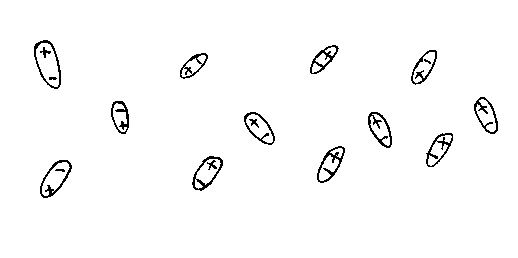
Then, let’s say you place a negative test charge in the center. The molecules then all suddenly point to the center negative charge with their positive end pointing to the negative charge.

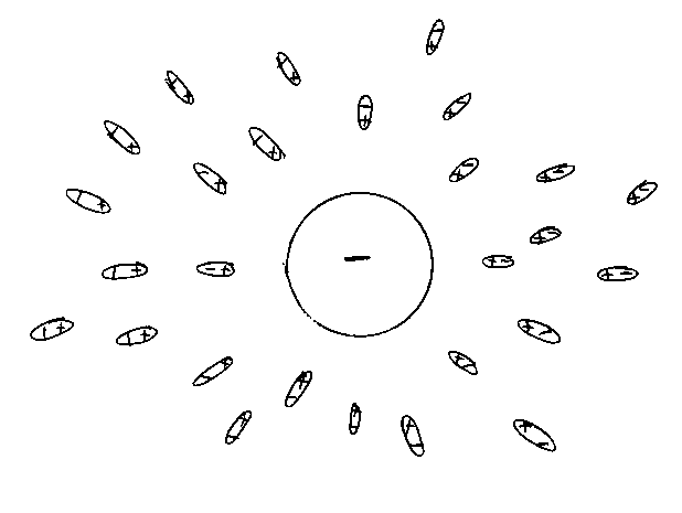
Now imagine a sphere surrounding this charge. There will be molecules that have one end sticking in the sphere, and the other end sticking out. The end sticking in the sphere will always be positive. Therefore, there will be slightly more positive charge than negative charge inside the sphere, not counting the center charge. The charge of the molecules inside the sphere will have a net positive charge. This positive charge will slightly off set the large negative charge in the center, so the total charge inside the sphere, including the center charge, will be slightly less negative than if there were no molecules. The larger the imaginary sphere, the more molecules will have their positive ends sticking in the sphere, and the more the center charge will be shielded. You could imagine a probe that measures charge located at the surface of the sphere. The measured charge of the center charge will increase as you get closer to the charge.

You have the same phenomenon if you try to measure the electric charge of an electron. In that case, it’s not surrounded by molecules with an electric dipole, but electron-positron pairs. However, they act the same way. As you get closer to an electron, its measured charge increases. This is called charge screening. A low-energy probe in the long range limit measures a value of the coulomb charge called the fine structure constant.

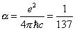
[alpha] = e²/4[pi][h bar]c = 1/137

In the past, people thought this number was of profound fundamental significance. Some people have tried to get this number by combining all sorts of other constants together, and claim it’s some sort of insight. Actually, this number is of no significance. The measured value of the coupling constant depends on the distance. The measured charge of an electron is higher closer to an electron. This has been confirmed experimentally. It is also believed that the coupling constants had different values in the early Universe, and originally all had the same value. This is called the running of the coupling constants.

A Landau pole in QED is a point at which the fine structure constant blows up as a function of the energy of the virtual photons being exchanged. In quantum field theory, the coupling constant for a particular force actually depends on an energy scale, which you can think of as the energy of the virtual particles being exchanged. For low-energy virtual photons, the fine structure constant is about 1/137, but at higher energies it gets bigger, and if there is a Landau pole, it actually becomes infinite. The existence of a Landau pole is usually taken as a sign that quantum electrodynamics breaks down when extrapolated to very high energies, which is the same as very short distance scales.

Now, you have the same phenomenon with quarks and color charge. A quark is surrounded by quark-antiquark pairs that shield its color charge. However, the gluons also have color, and they have the opposite effect. The gluons spread out the effective color of the quark. A red quark ends up being surrounded by other red charges, and so the measured red charge increases with distance. This is called antiscreening, and is the opposite of what happens with the electron.

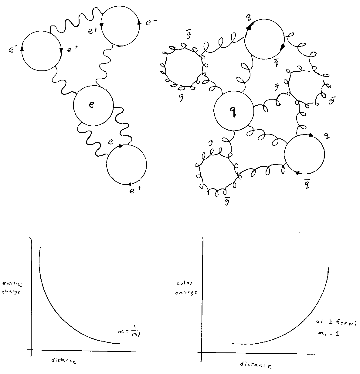
Because the effective charge of a quark increases with distance, this is why it’s not possible to pull quarks apart. Here you can see the electric field lines of an electron, and the color field lines of a quark.

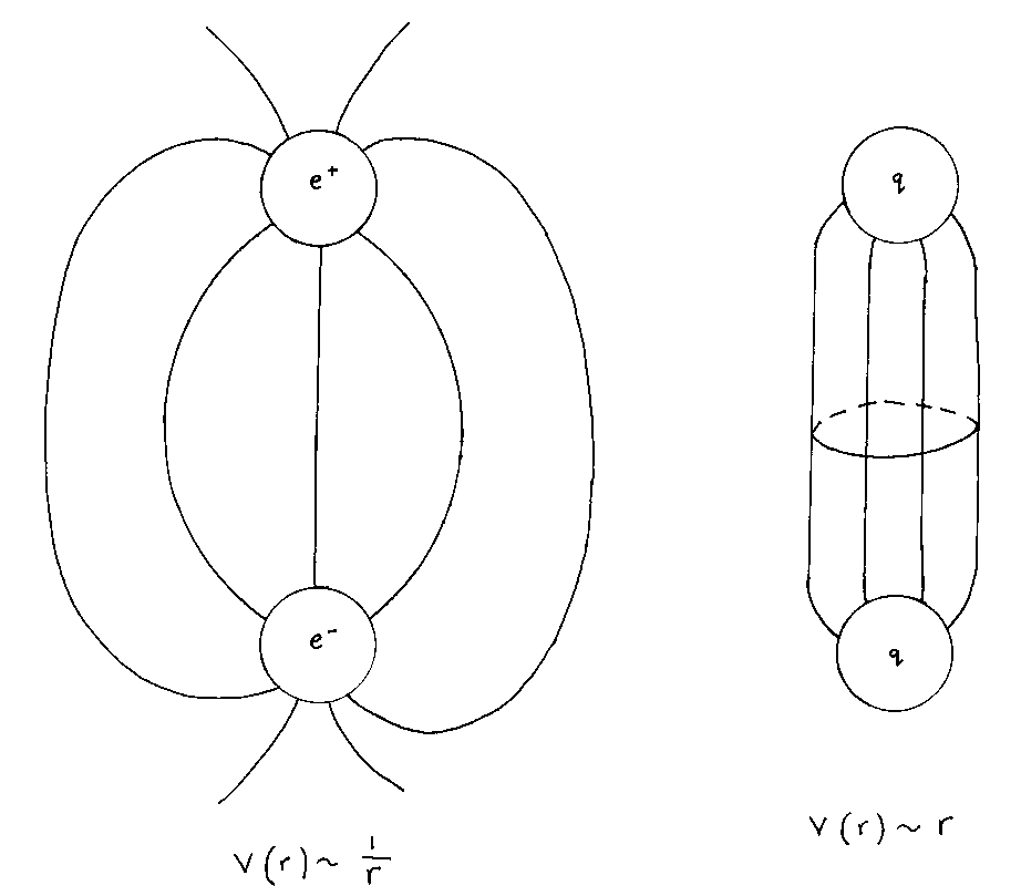
In the quark case, the field lines form a tube that increases in volume as the quarks are pulled apart. If you try to pull them apart, the energy bound up in this field becomes large enough to create other particles so it turns into other quarks, and so the quarks are never separated by much distance. If the distance between quarks increases, perhaps due to a collision in a particle accelerator, the force lines between them, which are sometimes called a color tube, increases in length until it breaks into smaller tubes with quarks at each end. This continues until the kinetic energy of the original quarks is converted into new quarks from which form the hadron jets seen in particle detectors at particle accelerators. Thus, you never see free quarks. This process is called confinement.

QCD and QED are very similar. The massless gluons exchanged between colored quarks are very similar to the massless photons exchanged between charged electrons. QCD has a more complex symmetry SU(3), rather than U(1). The main reason they act so different is simply that gluons are colored while photons are uncharged which causes the difference in the screening effects, and thus the measured magnitude of α and α_s.

Due to these effects, it’s very difficult to do calculations in QCD, especially at low energies. The equations are non-linear. Therefore we often resort to numerical computer simulations to get approximate results. The most successful method is called lattice QCD. Lattice QCD attempts to solve QCD problems by approximating spacetime with a discrete grid. Once they are put on a grid, these problems can be attacked by numerical methods on supercomputers. The approach was invented by Ken Wilson in 1974.

However, basically, quark-gluon interactions are computed with the rules of QED, using [squareroot of α_s] instead of [squareroot of α] at each vertex. It’s important to remember that QCD has been confirmed experimentally. In inelastic scattering experiments, analogous to Rutherford’s experiments, constituent partons within the proton can be detected that have been identified with quarks. Not only that, but we have detected electrically neutral partons that can be identified with gluons. A proton is two up quarks and a down quark. These are called the valence quarks. In addition, there are all the quark-antiquark pairs which are called the sea quarks.

I’m not going to show all of the Feynman rules for all of the possible lines and vertices involving quarks and gluons. You can only use the Feynman rules for QCD at high energy. At low energy, which is the same as large distances, the quarks are very strongly interacting, and you end up with confinement. At high energies, or short distances, the quarks are very weakly interacting, and you can use the Feynman rules for QCD to calculate the scattering amplitudes. Therefore, QCD is called an asymptotically free theory. In 1973, David Politzer, David Gross, and Frank Wilczek determined that QCD had this property of asymptotic freedom, meaning that at high energies, the particles are weakly interacting. They received the 2004 Nobel Prize in physics for their work.

In developing the quark model, the baryons and mesons were placed in multiplets that were arranged as hexagons, giant inverted triangles, or even pyramids. These diagrams illustrated the patterns in their quantum numbers, such as charge, isospin, baryon number, and strangeness. I could show them all but it would be too much of a digression so I’ll just give one simple example. The first studied hadrons, composed of up, down, and strange quarks, fit into octets of SU(3), and were therefore called “The Eight-Fold Way”. Later, higher representations, such as decuplets, were found. Gaps in the diagrams predicted new mesons and baryons, specifically the Ω^–, which consists of three strange quarks, similar to how gaps in the periodic table had predicted new elements. This shows the approximate SU(3) symmetry of up, down, and strange quarks in terms of how they combine to form mesons. It’s a meson octet plus a singlet. The x-axis is the third component of isospin, I₃, and the y-axis is hypercharge, B + S = Y. Also compare to the gluon colors which result from the exact color SU(3) symmetry.

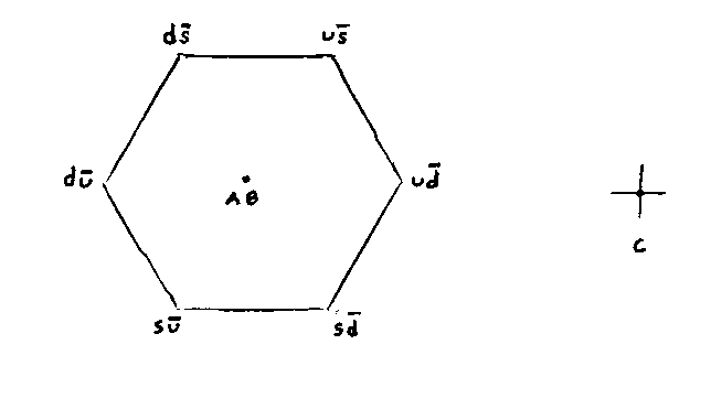
where

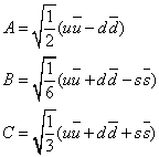
A = [squareroot of ½](u[u bar] – d[d bar])

B = [squareroot of 1/6](u[u bar] + d[d bar] + 2s[s bar])

C = [squareroot of 1/3](u[u bar] + d[d bar] + s[s bar])

Let’s look at the following two gluons.

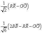
1/[squareroot of 2](R[R bar] – G[G bar])

1/[squareroot of 6](2B[B bar] – R[R bar] – G[G bar])

There is a 2-dimensional complex space of these gluons. The above two gluon states are orthogonal to each other, and are of unit size in this space. The colors and anticolors can be arranged in a hexagonal grid such that three directions correspond to colors, and the other three to anticolors. The gluon

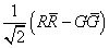
1/[squareroot of 2](R[R bar] – G[G bar])

causes R and R quarks to repel, G and G to repel, and R and G to attract. The gluon

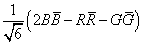
1/[squareroot of ](2B[B bar] – R[R bar] – G[G bar])

causes B and B to repel, R and R to repel, G and G to repel, B and R to attract, B and G to attract, and R and G to attract. Therefore, like charges repel and opposite charges attract. So if you had a red quark by itself, it would repel another red quark, and attract a blue and green quark, and form a baryon. The attractions and repulsions are a quantum interference effect between processes in which no gluons are exchanged, and those where a gluon is exchanged. If the gluon process has a minus sign in it, it attracts, otherwise, it repels.

In quantum mechanics, the probability that a particle is in a particular state is determined by squaring the absolute value of the amplitude for it to be in each of the possible states, and then adding up all the values. For the following gluon

1/[squareroot of 6](2B[B bar] – R[R bar] – G[G bar])

there is amplitude of

2/[squareroot of 6]

for it to be in a B[B bar] state, an amplitude of

1/[squareroot of 6]

for it to be in the G[G bar] or R[R bar] states. When you add them together, you get a probability of 1.

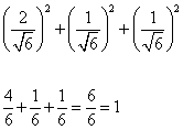
(1/[squareroot of 6])² + (1/[squareroot of 6])² + (1/[squareroot of 6])²

4/6 + 1/6 + 1/6 = 6/6 = 1

If the probabilities add up to 1, it’s called normalized, which is what you want. That’s why you include the 1/[squareroot of 2] and 1/[squareroot of 6] factors.

There are also the six other gluons that change the colors, and they can also attract and repel, due to quantum interference between processes where no gluons are exchanged, and processes where a gluon is exchanged. If the quarks are in the state

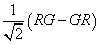
1/[squareroot of 2](RG – GR)

they will attract. If they are in the state

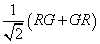
1/[squareroot of 2](RG + GR)

they will repel. In quantum mechanics, you can take quantum superpositions not only of single particle states, but all possible states. This is called entanglement. A quark in the 1/[squareroot of 2](RG – GR) is the same as an antiblue quark.

The six gluons can’t be distinguished from the other two gluons because the SU(3) symmetry mixes them with each other. For instance, one of the symmetries of SU(3) is that it is the same if you replace R with 1/[squareroot of 2](R + G), and replace G with 1/[squareroot of 2](G – R). The SU(3) has eight dimensions, same as the number of gluons, and thus there are many different ways to mix the different colors of quarks. If you take the following gluon

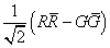
1/[squareroot of 2](R[R bar] – G[G bar])

and the result of the transform is

½[squareroot of 2](R + G)([R bar] – [G bar]) – ½[squareroot of 2](G – R)([G bar] – [R bar])

which is the same as

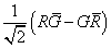
1/[squareroot of 2](R[G bar] + G[R bar])

so therefore the two gluons can be thought of as a superposition of the other six gluons. There is no distinction between the six gluons that change the colors of quarks, and the two other gluons, because they are mixed together by the SU(3) transform. They are all within the 8-dimensional representation of SU(3). The two gluons don’t interact with each other because they have the same colors as anticolors, but they do interact with the other six gluons, and thus do have color charge.

In electromagnetism, if the charges balance out in positives and negatives, the result is neutral, but that’s not true for the strong force. A particle is only neutral in a force if it is unaffected by the symmetry the force is based on. Therefore, a red-antired meson is not color neutral because the symmetry saying R and G are the same mixes it with, say, the green-antigreen meson. The only color neutral meson combination is

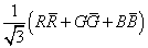
1/[squareroot of 3](R[R bar] + G[G bar] + B[B bar])

The only color neutral baryon combination is

1/[squareroot of 6](RGB – RBG + GBR – GRB + BRG – BGR)

If a particle is composed of constituent particles, the constituent particles can exchange bosons that cause them to turn into other particles. As a result, the overall particle they had previously comprised will decay into other particles. The strength of the force involved has a great effect on the time it takes the overall particle to decay. Here is a typical decay via the strong force.

[delta] -> p[pi]

which has a lifetime of 10^-23 seconds. There are also decays via electromagnetic interaction such as

[sigma] -> [lambda][gamma]

which have decays in the 10^-20 – 10^-16 seconds range. This is what you would expect if

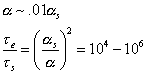
[alpha] ~ .01[alpha]_s

[tau]_e/[tau]_s = ([alpha]_s/[alpha])² = 10⁴ – 10⁶

However, this does not explain much longer lifetimes. There are some particles that have a lifetime of 10^-12 seconds or more. An example is

[pi]^– -> e + [nu bar]

which has a lifetime of 10^-12 seconds. However, the most extreme example is the decay of the neutron.

n -> p + e + [nu]

This is called beta decay. The neutron has a lifetime of 15 minutes! Obviously, this can’t be explained by either electromagnetism or the strong force. It has to be a new force. This new force is weaker than the strong force or electromagnetism, so it was called the weak force.

Based on the difference in the lifetimes, the coupling constant for the weak force would be

[alpha]_w = 10^-6 [alpha]_s

Unlike the strong force, the weak force acts on both leptons and quarks. Also, the weak force can change a down quark into an up quark, or a muon into a neutrino. The weak interactions change the quark and lepton flavor.

In 1934, Enrico Fermi thought up a Lagrangian for the weak interaction. The fermion current is

J^u = [psi bar] [gamma]^u [psi]

The Lagrangian has to be a product of four fermion fields.

[psi bar]_p [psi]_n [psi bar]_e [psi]_[nu]

If these contain creation and annihilation operators, the lowest order processes then describe beta decay. Fermi came up with the following Hamiltonian.

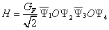
H = (G_F/[squareroot of 2) [psi bar]₁ O [psi]₂ [psi bar]₃ O [psi]₄

where G_F is the Fermi constant. When Fermi originally wrote this, he defined O to be consistent with Lorentz invariance and parity symmetry. Then, in 1956, in order to explain τ – θ, Lee and Yang suggested that weak interactions do not conserve parity. In 1957, this was experimentally confirmed by Wu, Amber, Hayword, and Hobson in the decay of polarized Co⁶⁰. Then in 1957, Marshak, Sudarshan, Feynman, Gell-Mann, and Sakurai suggested the following form

O = [gamma]^u (1 + [gamma]⁵)

This gives an axial vector. Therefore, the interaction is called vector – axial vector, or V – A. The Fermi Lagrangian then takes the following form.

L = -(G_F/[squareroot of 2]) [[psi bar]_p [gamma]^u (1 – g[gamma]⁵) [psi]_n] [[psi bar]_e [gamma]_u (1 – [gamma]⁵) [psi]_[nu]]

Since he derived this for protons and neutrons, which we now know are not fundamental, g = 1.26. For quarks, g = 1. G_F is the Fermi constant.

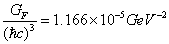
G_F/([h bar]c)³ = 1.166 x 10^-5 GeV^-2

The Fermi Lagrangian contains γ⁵ which violates parity. Therefore, the Fermi Lagrangian is only capable of creating neutrinos with left-handed helicity. This does not mean that right-handed neutrinos are impossible, only that they are created in tiny amounts since the neutrino’s mass is so small.

Fermi’s theory is not renormalizable. The diagram for muon decay would be

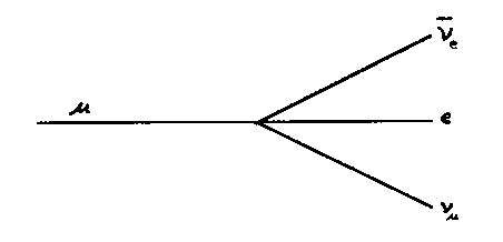
We know this can’t be right since there is no boson mediating the force. He essentially imagined that the boson had infinite mass so it’s range was zero, and thus didn’t exist. In this version, the coupling constant is in units of [energy]^-2 instead of dimensionless.

In order to get a renormalizable theory, you should instead use

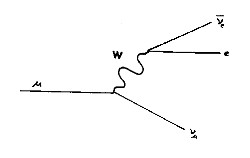
Even then, it’s only renormalizable if m_W = 0. However, if that were true, it would be of infinite range, which it is not. Later, this was explained using the Higgs mechanism.

The weak interaction is described by an SU(2) symmetry. Particles can be grouped into doublets of particles that differ by one unit of charge.

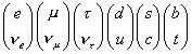
Therefore, the emission or absorption of a particle with a charge of +1 or -1 can cause a particle to change into the other particle in its doublet. These particles with charge of +1 and -1 are called the intermediate vector bosons, and are symbolized by W⁺ and W^–.

The symmetry suggests the following transformation.

[psi] -> e^i[theta]M

where M is a 2 x 2 matrix. The generators must be Hermitian and traceless, corresponding to SU(2), and therefore must be the Pauli spin matrices. If the weak force Lagrangian is invariant under SU(2) transformations, the group element

g = 10^[theta]_iG_i

shows that each of the three generators G_i is associated with an arbitrary angle θ_i. Remember before, we added a field identified with the photon to make it locally invariant. Here, it’s the same, except you have to hide three angles. Therefore, you have to add not one or two but three gauge fields to hide these angles. That means there must exist a third intermediate vector boson in addition to the two we already know about. This is the Z⁰ intermediate vector boson which is electrically neutral.

You might expect the following transformation to ensure gauge invariance.

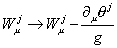
W_u^j -> W_u^j – ([partial derivative]_u[theta]^j)/g

However, this will not work because the group is non-Abelian. You must therefore have the following transformation.

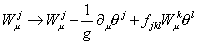
W_u^j -> W_u^j – (1/g)[partial derivative]_u[theta]^j + f_jklW_u^k[theta]^l

where f_jkl are the structure constants. For SU(2), the generators are Pauli spin matrices, and the structure constants are ε_ijk.

This transformation law for non-Abelian gauge fields causes the kinetic part of the Lagrangian to take the following form.

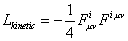
L_kinetic = -(1/4) Fⁱ_uv F^iuv

where

Fⁱ_uv = [partial derivative]_uW_v^j – [partial derivative]_v W_u^j – g f_jkl W_u^kW_k^l

This means that the gauge bosons can self-interact.

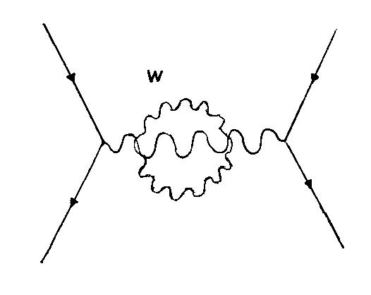
You can think of the fields and particles as being created by other fields combining in a certain way. For instance, the photon is considered to be a fundamental particle but the electromagnetic field A_u can be considered to be the result of two other fields, W_u and B_u. This is not to say that photons or the electromagnetic field are made of something else, but that mathematically, it can be described that way.

The boson fields of the weak force are W_i^u, where i = 1, 2, 3 and they combine in the following ways to form the following particles.

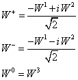
W⁺ = (-W¹ + iW²)/[squareroot of 2]

W^– = (-W¹ – W²)/[squareroot of 2]

W⁰ = W³

There is no particle called W⁰ but later this field will combine with the B_u field to create the electromagnetic field A_u and the Z⁰. Compare with the pion isospin states I gave earlier. Before that, however, I want to write down the Standard Model Langrangian.

Separate the electron into right-handed and left-handed types.

e^–_R = P_R [psi]_e

e^–_L = P_L [psi]_e

The right-handed electron is placed in an SU(2) singlet. The left-handed electron and the electron neutrino, which is always left-handed, is placed in an SU(2) doublet.

Similarly, the left-handed up and down quarks are put in a doublet, while the right-handed up and down quarks are put in singlets.

Thus, the Standard Model Lagrangian is

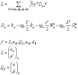
L = [summation, f = L, e_R, Q_L, u_R, d_R] [f bar] i[gamma]^u D_u f

where D_u = [partial derivative]_u – ig₁(Y/2)B_u – ig₂([tau]ⁱ/2)W_uⁱ – ig₃([lambda]^a/2)G_u^a

f = L, e_R, Q_L, u_R, d_R

L = ([nu]_e e)_L Q_L = (u, d)_L

and where Y is the hypercharge, τⁱ are the Pauli spin matrices, λ^a are the Gell-Mann matrices, and g₁, g₂, and g₃ are coupling constants.

We say that the electromagnetic field A_u is a combination of B_u and of W_u⁰ which are orthogonal normalized fields.

A_u is proportional to g₂ B_u – g₁ Y_L W_u⁰

A_u is orthogonal to another field Z_u

Z_u is proportional to g₁ Y_L B_u + g₂W_u⁰

Then A_u and Z_u are defined as follows.

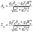
A_u = (g₂B_u – g₁Y_LW_u⁰)/[squareroot of (g₂² + g₁²Y_L²)]

Z_u = (g₁Y_LB_u + g₂W_u⁰)/[squareroot of (g₂² + g₁²Y_L²)]

You can then solve for B^u and W_u⁰

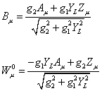
B^u = (g₂A_u + g₁Y_LZ_u)/[squareroot of (g₂² + g₁²Y_L²)]

W_u⁰ = (-g₁Y_LA_u + g₂Z_u)/[squareroot of (g₂² + g₁²Y_L²)]

I want to avoid algebra in this paper so I’ll just give the results. You can also solve for e, the charge of the electron. You ultimately get

e = (g₁g₂)/[squareroot of g₂² + g₁²]

You can then define

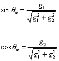
sin [theta]_w = g₁/[squareroot of g₂² + g₁²]

cos [theta]_w = g₂/[squareroot of g₂² + g₁²]

and thus

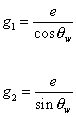
g₂ = e/(sin [theta]_w)

g₁ = e/(sin [theta]_w)

where θ_w is the Weinberg angle.

sin² [theta]_w ~ 0.23

So ultimately, you have the W^u fields which mix to create the W⁺ and W^–. The W^u field combines with the B^u field in one way to create the electromagnetic field A_u, and in another way to create the Z⁰.

Here are some numerical relations for the few GeV range and below.

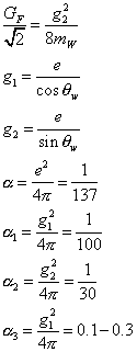
G_F/[squareroot of 2] = g₂²/8m_W

g₂ = e/sin [theta]_w

g₁ = e/cos [theta]_w

[alpha] = e²/4[pi] = 1/137

[alpha]₁ = g₁²/4[pi] = 1/100

[alpha]₂ = g₂²/4[pi] = 1/30

[alpha]₃ = g₃²/4[pi] = 0.1 – 0.3

This combination of electromagnetism and the weak force is called electroweak theory. It was first suggested by Sheldon Glashow in 1961. It was then elaborated by Steven Weinberg in 1967, and Abdus Salam in 1968. Glashow, Weinberg, and Salam shared the 1979 Nobel Prize for their work. Steven Weinberg’s 1967 paper unifying electromagnetism and the weak force is the most frequently cited paper in Physical Review Letters. Weinberg and Salam added the concept of mass generation via the Higgs mechanism. The electroweak theory works fine except that it assumes the intermediate vector bosons were massless, which would cause the weak force to be a long range force, which it is not. If they were massive, it would be a short range force. How do you add mass without destroying the gauge invariance? This is accomplished by the Higgs mechanism.

The electroweak is a SU(2) x U(1) theory. The Lagrangian density of the boson is a sum of the U(1) gauge fields B_u, and the three SU(2) gauge fields W_uⁱ, where i = 1, 2, 3.

L = -(1/4) F_Buv (x) F_B^uv – (1/4)F_Wuvⁱ (x) F_W^iuv (x)

where

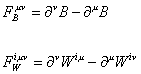
F_B^uv = [partial derivative]^vB – [partial derivative]^uB

F_W^iuv = [partial derivative]^vW^iu – [partial derivative]^uW^iv

The familiar fields are formed by

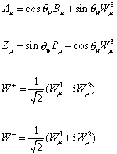
A_u = cos [theta]_w B_u = sin [theta]_w W_u³

Z_u = sin [theta]_w B_u – cos [theta]_w W_u³

W⁺ = 1/[squareroot of 2]/(W_u¹ – iW_u²)

W^– = 1/[squareroot of 2]/(W_u¹ + iW_u²)

Now you could just include mass terms for the W⁺, W^–, and Z⁰ particles but then it would no longer be invariant under U(1) gauge transformations.

[psi](x) -> [psi]'(x) = e^iY[xi](x)[psi](x)

where Ψ is the boson field, Y is the hypercharge, and ξ(x) is any differentiable function.

The way you give mass to the W and Z bosons while keeping the gauge theory SU(2) x U(1) invariant is by spontaneous symmetry breaking.

The easiest way to describe this concept is with the Mexican hat potential. Let’s say you had a system where the minimum energy was not at the origin. You could imagine a classical system with a small ball placed on top of a hill.

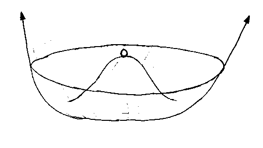
On top of the hill, the ball is at the origin, and the system is symmetric under rotations about the z-axis. However, it is unstable. The ball is not at minimum gravitational potential energy. Now, if the ball were to roll down the hill to the ring at the bottom, the system would no longer be symmetric under rotations about the z-axis. However, the ball would now be in a state of minimum gravitational potential energy. It’s now in an energetically favorable position. This is spontaneous symmetry breaking at the classical level.

Another frequently cited example of spontaneous symmetry breaking involves ferromagnetism, but I think the above simple example is actually a better analogy for the Higgs mechanism.

Let’s do a simple example before doing the Higgs mechanism. Let’s say you have the following example.

L = [partial derivative]^u [psi]* [partial derivative]_u [psi] – V([psi])

where Ψ is a complex field

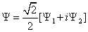
[psi] = ([squareroot of 2]/2) [[psi]₁ + i[psi]₂]

and V(Ψ) is the potential energy

V([psi]) = [mu]² | [psi] |² + [lambda] | [psi] |⁴

The constants μ² and λ are real, with λ positive so it will be bounded from below. The Lagrangian is invariant under global U(1) transformation describing rotations in the complex plane. In order for the vacuum, the lowest energy state, to be invariant under Lorentz transformations and translations implies that Ψ (x) is a constant in the vacuum state.

If μ² is positive, then the minimum potential energy is when Ψ = 0. If μ² is negative, the minimum potential energy is a ring in the complex plane.

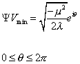
[psi] V_min = [squareroot of -[mu]²/2[lambda]] e^i[theta]

It doesn’t make any difference what direction it goes in, so let’s set θ = 0

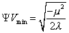
[psi] V_min = [squareroot of -[mu]²/2[lambda]]

Define ν such that

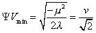
[psi] V_min = [squareroot of -[mu]²/2[lambda]] = v/[squareroot of 2]

The deviation from the chosen minimum can be described in terms of the real fields σ and n defined by

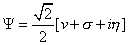
[psi] = ([squareroot of 2]/2) [v + [sigma] + in]

The Lagrangian written in terms of σ and n is

L = (1/2) [partial derivative]^u [sigma] [partial derivative]_u – [lambda]v²[sigma]² + (1/2)[partial derivative]^un[partial derivative]_un – [lambda]v[sigma][[sigma]² – n²] – (1/4)[lambda][[sigma]² + n²]² + C

The higher terms are interaction terms so the free Lagrangian is

L = (1/2) [partial derivative]^u [sigma] [partial derivative]_u – [lambda]v²[sigma]² + (1/2)[partial derivative]^un[partial derivative]_un

σ and n are two real Klein-Gordon fields. By quantizing these fields, the Lagrangian describes two different spin 0 particle fields. The σ bosons will have mass

m_[sigma] = v[squareroot of 2[lambda]]

arising from the σ² while the n bosons are massless due to the minimum being degenerate. The remaining terms are interactions among the σ and n through perturbation theory.

In this hypothetical example, the spontaneous symmetry breaking of the U(1) symmetry, caused by the degenerate energy minimum of the Lagrangian, created a perturbation theory with a massive scalar boson.

Next, I’ll show the Higgs mechanism for a U(1) x SU(2) theory. You replace the normal derivative with the covariant derivative

D_u = [partial derivative]_u + iqA_u

You add the Lagrangian of the free fields.

L = D^u [psi]* D_u [psi] – V([psi]) – (1/4)F_uvF^uv

This new Lagrangian is invariant under the U(1) gauge transformation.

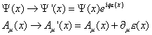
[psi](x) -> [psi]'(x) = [psi](x)e^iq[xi](x)

A_u -> A_u‘(x) = A_u(x) + [partial derivative]_u [xi](x)

where ξ is any differentiable function. You continue the same way we did before, and express the Lagrangian in terms of the variables σ and n.

L = (1/2)[partial derivative]^u[sigma][partial derivative]_u[sigma] – [lambda]v²[sigma]² + (1/2)[partial derivative]^un[partial derivative]_un -(1/4)F_uvF^uv + (1/2)q²v²A_uA^u + qvA^u[partial derivative]_un + higher terms

The Lagrangian has a massive vector boson field A and two scalar boson fields σ, n, with n massless. However, it also has the term

A^u[partial derivative]_un

There is no way to interpret this. It is not an interaction term since it is quadratic in the fields as if it were a free field. Therefore, we have to get rid of it. This Lagrangian has an extra degree of freedom that can be absorbed by doing a gauge transformation where

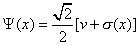
[psi](x) = ([squareroot of 2]/2) [v + [sigma](x)]

In this gauge, the n field disappears, leaving

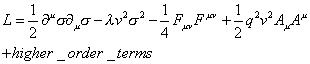
L = (1/2)[partial derivative]^u[sigma][partial derivative]_u[sigma] – [lambda]v²[sigma]² + (1/4)F_uvF^uv + (1/2)q²v²A_uA^u + higher terms

The way the Higgs mechanism works is that when you have symmetry breaking, the number of degrees of freedom doesn’t change, but the particles change, so the degrees of freedom are redistributed into other particles. This only works if you have a degenerate vacuum.

Let’s see how the numbers work out. A scalar particle has one degree of freedom. A complex scalar field has two degrees of freedom since a + bi has two components. A massless vector particle travels at the speed of light, so it only has two transverse polarized states, so that’s two degrees of freedom. A massive vector particle also has a longitudinal polarized state, so that’s three degrees of freedom.

In our first simple example of U(1) spontaneous symmetry breaking, before symmetry breaking, you had a complex scalar field (2 degrees of freedom), and a massless vector boson (2), so that’s 2 + 2 = 4. After symmetry breaking, you had a scalar particle (1), and massive vector boson (3), so that’s 1 + 3 = 4.

In the recent case of the U(1) x SU(2) Higgs mechanism, before symmetry breaking, you had a complex doublet (2 + 2 = 4), and four massless vector bosons (2 + 2 + 2 + 2 = 8). Therefore you had 4 + 8 = 12 degrees of freedom. After symmetry breaking, you had a scalar particle (1), a massless vector boson (2), and three massive vector bosons (3 + 3 + 3 = 9). Therefore you had 1 + 2 + 9 = 12 degrees of freedom.

The three massive vector bosons are the W⁺, W^–, and Z⁰. The massless vector boson is the photon. The scalar particle is the Higgs particle.

Introducing the masses of the vector bosons with one complex doublet of complex scalars is the simplest scenario. An infinite number of such scalar fields can be added. The simplest supersymmetric models have five scalar fields left over after the Higgs mechanism. They are a doublet of charged scalars, two neutral scalars, and one neutral psuedoscalar.

The masses of the particles are given by

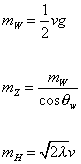
m_W = (1/2)vg

m_Z = m_W/cos [theta]_w

m_H = [squareroot of 2[lambda]v]

where g is the weak coupling constant, and θ_w is the Weinberg angle. You can express m_W and m_Z through G_F, α, and sin θ_w by using the following relations

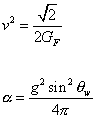
v² = [squareroot of 2]/2G_F

[alpha] = (g²sin²[theta]_w)/4[pi]

where G_F is the Fermi constant, and α is the fine structure constant. You can measure the Fermi constant from the muon lifetime, and the Weinberg angle from the relative cross sections of the neutral current and charged current. It was therefore possible to predict the masses of the W⁺, W^–, and Z⁰. In 1983, these three particles were detected with the expected masses in the UA1 and UA2 experiments at the CERN proton-antiproton synchrotron.

The vacuum expectation value is

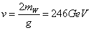
v = 2m_W/g = 246 GeV

We have no way of measuring λ so we have no way of calculating the Higgs mass. However, self-consistency sets an upper limit on the Higgs mass of 1 TeV. Right now, the search for the Higgs particle is the primary focus of experimental particle physics.

The Lagrangian for the electroweak and Higgs is divided into the following sections.

L = L₀ + L_FB + L_FH + L_BB + L_BH + L_HH

L₀ is the Lagrangian of the free fields

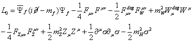
L = [psi bar]_f (i[partial derivative slash] – m_f)[psi]_f -(1/4)F_uvF^uv -(1/2)F_uv^dagF_w^uv +m_W²W_u/^dagW^u -(1/4)F_zuvF_z^uv + (1/2)m_Z²Z_uZ^u + (1/2)[partial derivative]^u[sigma][partial derivative]_u[sigma] – (1/2)m_H²[sigma]²

L_FB is the interaction between fermions and bosons, L_FH between fermions and Higgs, L_BB between bosons and bosons, L_BH between bosons and Higgs, and L_HH is the Higgs self-interaction.

Here is the fermion Higgs interaction term.

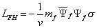
L_FH = -(1/v)m_f [psi bar]_f [psi]_f [sigma]

When a symmetry is spontaneously broken, you get a massless particle called the Nambu-Goldstone boson. Also called just a Goldstone boson, named after Jeffrey Goldstone, it is a massless boson resulting from a spontaneously broken global symmetry. Now, you might initially assume that the Higgs boson is such a particle but actually it is not. In field theories where local symmetries are spontaneously broken by the vacuum, the massless particles do not appear in the spectrum of physical states but rather provide longitudinal modes to the gauge bosons which become massive. Massless particles have just two transverse polarized states. When the W⁺, W^–, and Z⁰ become massive, they gain a longitudinal state, which is actually the Goldstone boson associated with the symmetry breaking.

During symmetry breaking, the Hilbert space contains a physical subspace and an unphysical subspace. The Goldstone boson, and the massless gauge fermions, remain in the unphysical subspace, but their linear combination has extensions in the physical subspace, which is the resulting massive bosons.

The full name of the Higgs mechanism is actually the Brout-Englert-Higgs-Guralnik-Hagen-Kibble mechanism. Obviously, that’s a cumbersome name, so they just name it after Peter Higgs.

Fermions can scatter by exchanging Higgs like other bosons but this is not considered a separate force because it does not have its own coupling constant, and is derived from the electroweak.

On 4 July 2012, the ATLAS and CMS experiments at CERN’s Large Hadron Collider announced they had each observed a new particle in the mass region around 126 GeV. This particle is consistent with the Higgs boson predicted by the Standard Model. The Higgs boson, as proposed within the Standard Model, is the simplest manifestation of the Brout-Englert-Higgs mechanism. Other types of Higgs bosons are predicted by other theories that go beyond the Standard Model.

There is a major flaw with the Standard Model as described so far which I have not mentioned. According to the Standard Model Lagrangian previously given, all of the fermions are massless! Obviously, you can’t just add mass terms since that would destroy gauge invariance. Luckily, the Higgs mechanism comes to the rescue. The Higgs mechanism does not give masses to the fermions the way it does for the W⁺, W^–, and Z⁰, but the interaction between the fermion fields and the Higgs complex scalar field allows for fermion masses.

Let’s say you have the following interaction Lagrangian for leptons. The second term is a Hermitian conjugate of the first.

L_int = g_e ([L bar] [phi]e_R + [phi] ^†[e_R bar]L)

where the lepton doublet is

and the Higgs complex doublet is

The following equation is SU(2) invariant.

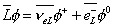
[L bar] [phi] = [nu bar]_eL[phi] ^† + [e_L bar][phi]⁰

Multiplying by the singlet e^–_R has no effect on SU(2) invariance. The coupling g_e is arbitrary.

Now let’s say spontaneous symmetry breaking takes place. Then you make the following substitution.

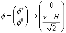
where v is the Higgs vacuum expectation value, and H is the remaining physical Higgs boson. You then get

L_int = (g_ev/[squareroot of 2])([e_L bar]e_R + [e_R bar]e_L) + (g_e/[squareroot of 2])([e_L bar]e_R + [e_R bar]e_L)H

The first term in the Lagrangian can be identified with the fermion mass. You can then write the electron mass as

m_e = g_ev/[squareroot of 2]

Now, if it were possible to somehow measure g_e experimentally, then the Standard Model would be able to actually calculate fermion masses similar to calculating the masses of the intermediate vector bosons. However, we have no idea how to do that, so instead the Standard Model simply allows for the existence of fermion masses without calculating them. The only way to get a value for g_e is to measure the electron mass, and use that to calculate it.

g_e = ([squareroot of 2]m_e)/v

The second term in the Lagrangian says there is an electron-electron-Higgs vertex of strength

g_e/[squareroot of 2] = m_e/v

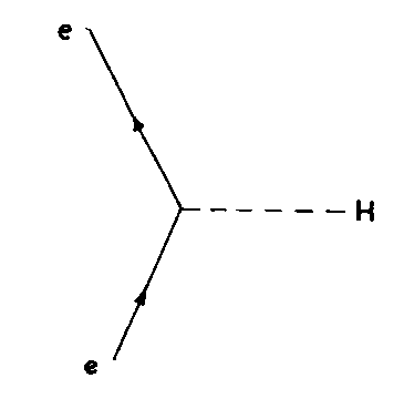
Rewriting the interaction Lagrangian to eliminate g_e, you have

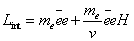
L_int = m_e [e bar]e + (m_e/v) [e bar]eH

For quarks, it proceeds as above, but with an additional element which didn’t exist before since there is no ν_R.

In SU(2) spin theory, if

is an SU(2) doublet, then so is

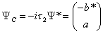
Similarly, if

is an SU(2) doublet, then so is

which after spontaneous symmetry breaking, becomes

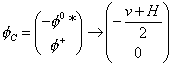
Since φ has hypercharge Y = +1, φ₀ has Y = -1, and still satisfies Q = I₃ + Y/2.

Then for quarks

L_int = g_d[Q_L bar][phi]d_R + g_u[Q_L bar][phi]_cu_R + Hermitian conjugate

After going through algebra, you get

L_int = m_d[d bar]d + m_u[u bar]u + (m_d/v)[d bar]dH + (m_u/v)[u bar]uH

Thus, the theory allows for up and down masses but does not calculate them, since we have no way of knowing g_u or g_d. The last two terms are interaction terms between the down quark and the Higgs, and the up quark and the Higgs.

Like everything else in the Standard Model, the second and third generations of fermions are identical to the first except for the measured value of the masses. They are handled in the same way.

The above method for allowing masses for the fermions can not be used for the neutrinos since according to the Standard Model, there are no right-handed neutrinos, or at least they don’t appear in the doublets. Therefore, for a long time, it was assumed that neutrinos were massless. Then in the late 1970’s, there was some experimental evidence, which later turned out to be inaccurate, that neutrinos were massive, and it got people thinking about the idea. Since then, there has been a steady increase in the evidence to support the claim until today, it’s assumed that neutrinos have a small mass. Here are some reasons to think so.

1. Just the pattern of the Standard Model. The fermions are massive, and the bosons are massless. You could make the claim that the intermediate vector bosons were originally massless, and later acquired a mass via the Higgs mechanism.

2. The Solar Neutrino Problem. We detect fewer electron neutrinos from the Sun than we should which can be explained by neutrino oscillation, where neutrinos of one type turn into neutrinos of another type. This is only possible if they have mass.

In 1969, Bruno Pontecorvo suggested that neutrinos might oscillate between the electron and muon flavor states. Oscillations can occur if the physical neutrinos are actually particles with different masses but not unique flavors. An electron neutrino can change into a muon neutrino or tau neutrino as they propagate because the mass components that made up that pure flavor get out of phase. The probability for neutrino oscillations are enhanced as neutrinos interact with first generation fermions while leaving the Sun. This effect of matter-enhanced neutrino oscillations is called the MSW effect, developed by Mikheyev, Smirnov, and Wolfenstein in 1985. The measurements at the Sudbury Neutrino Observatory showed that the neutrino flux produced in the beta decay reaction in the Sun contains a significant non-electron type component when measured on Earth. This measurement is strong indication for the oscillation of solar neutrinos. This is strong evidence that neutrinos have mass.

3. Dark Matter. Massive neutrinos could be a hot dark matter candidate to help explain dark matter.

4. Supernovae 1987A. The neutrinos from the supernovae arrived at Earth over an interval of time. If they were massless, they would all be traveling at the speed of light, and would arrive simultaneously.

Thus neutrinos are believed to have a small mass but they can’t be given mass by the same method described above for the other fermions. One simple way to allow neutrino masses is to take the lepton doublet and the Higgs doublet to write the following Lagrangian.

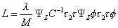
L = ([lambda]/M)[psi]_L C^-1 [tau]₂ [psi]_L [phi] [tau]₂ [tau][phi]

where M is a new mass scale with M >> m_W. The presence of 1/M is to give the operator the correct dimension. After SU(2) x U(1) symmetry is broken, you get the following effective mass for the neutrino.

M_[nu]e = (4m_W²/g²M)[lambda]

Another method of generating neutrino masses is called the seesaw mechanism, and is realized in Grand Unified Theory models. The neutrino mass is a combination of the Dirac and Majorana forms.

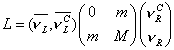
The Dirac mass m is generated the same way as the lepton masses. The mass M is large enough to explain why right-handed neutrinos are not seen since M is of the order of the GUT mass. The seesaw mechanism predicts the scaling

m_[nu]e : m_[nu][mu] : m_[nu][tau] = m_u² : m_c² : m_t²

What I described earlier was the minimal Higgs model with a single complex doublet. The next simplest possibility is to imagine two Higgs doublets which can be used to solve the strong CP problem.

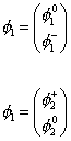
The W and Z boson masses receive a contribution from both vacuum expectation values.

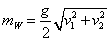
m_W = (g/2)[squareroot of v₁² + v₂²]

In this case, there are three neutral Higgs bosons, a positive Higgs, and a negative Higgs that remain physical after spontaneous symmetry breaking.

This model has an extra chiral U(1) symmetry which is identified with the U(1)_PQ symmetry which is one possible solution to the strong CP problem.

Before when I discussed QCD, I ignored one additional possible gauge-invariant contribution to the Lagrangian which takes the following form

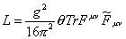
L = (g²/16[pi]²) [theta] Tr F^uv [F tilde]_uv

where the dual field tensor is

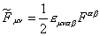
[F tilde]_uv = (1/2)[epsilon]_{uv[alpha][beta]}F^{[alpha][beta]}

ε is a pseudotensor that changes sign under reflection. Therefore, the term causes CP violation.

The observed amount of CP violation is very small. From limits on a possible magnetic moment of the neutron, we have

| [theta] | < 10^-9

We do observe CP-violation due to the weak force. Weak CP-violation is contained in phases of the elements of the KM-matrix. However, we do not observe the QCD induced CP-violation predicted by the Standard Model, and this is called the strong CP problem. In 1977, Roberto Peccei and Helen Quinn suggested a possible solution to the strong CP problem. They theorized a new symmetry called Peccei-Quinn symmetry. This is an axial version of a simple phase rotation.

q -> e^{i[beta][gamma]5}q

[phi] -> e^-2i[beta][phi]

The transformation of the Higgs field is needed to keep QCD invariant. The effect of breaking this symmetry is to add a term in the Lagrangian of the same form as the CP-violating term but in which θ is now the phase of φ. The breaking of the Peccei-Quinn symmetry, which is global, creates a Goldstone boson called the axion. Even though Goldstone bosons are normally massless, the axion can acquire a small mass. Therefore the axion is a prime candidate for cold dark matter.

There is an extra global chiral U(1) symmetry called U(1)_PQ which is spontaneously broken. The axion arises as the pseudo-Nambu-Goldstone boson for the broken symmetry. It’s called “pseudo” because the U(1)_PQ symmetry is anomalous. This is what causes it to have mass. It has both QCD and electromagnetic anomalies, so you get a coupling to two photons. An axion in a background magnetic field could convert to a photon. Axions could also carry energy away from stars, so this gives another constraint. Other constraints come from looking for reactions like K⁺ → π⁺ + axion. The original Peccei-Quinn model had the U(1)_PQ breaking associated with electroweak symmetry breaking, and is ruled out experimentally. Now the interest is in invisible axion models where the U(1)_PQ breaking scale is much higher. The axion mass equals λ_QCD^{2}/f, where f is the PQ breaking scale, so invisible axions are very light. Current limits still leave the axion as a very good candidate for cold dark matter.

CP-violation was discovered in 1964 by Christenson, Cronin, Fitch, and Turlay in K⁰ decays. The kaon is an u[s bar] meson, and for a long time, they were the only systems where CP-violation was observed. The neutral kaon K⁰ and it’s antiparticle [K bar]⁰ form a CP-even state (K⁰ + [K bar]⁰)/[squareroot of 2], which decays into two pions, and a CP-odd state (K⁰ – [K bar]⁰)/[squareroot of 2], which decays into three pions, the rate of which is suppressed by the much smaller phase space available for the decay. CP-symmetry explained the large difference in lifetimes of the two neutral K mesons. However, in 1964, James Christenson, James Cronin, Val Fitch, and Rene Turlay observed the decay of the long-lived K meson into two pions. The CP-odd state therefore had a small admixture of the CP-even state. If the mass eigenstates are not CP eigenstates, that means CP-symmetry is violated. Since we assume particle physics is CPT-invariant, CP-violation must imply T-violation. One way of looking for CP-violation is to look for kinematical effects odd under time-reversal invariances. In 2000, there was finally observed some indication of CP-violation in the decay of the B meson.

The Fermi constant deduced from neutron beta decay is slightly smaller than the Fermi constant deduced from muon decay. This is because the up, down and strange quarks interacting by the weak force are not flavor eigenstates but are rotated by a mixing angle, θ_c, called the Cabibbo angle. This was invented by Nicola Cabbibo in 1963, when the up, down, and strange quarks were the only quarks known. Therefore, the flavors of quarks recognized by the strong force interaction are not exactly the same as those recognized by the weak interaction. Actually, they are linear combinations. Here is the Fermi Lagrangian.

L = (G_F/[squareroot of 2]) J^uJ_u^†

where

J^u = [u bar][[gamma]^u (1-[gamma]⁵)]d’ + [c bar][[gamma]^u(1-[gamma]⁵)]s’

where you have the following rotations

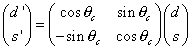
where θ_c is the Cabbibo angle. θ_c ~ 13°.

When the up, down, and strange quarks were the only quarks known, there was the problem that the K⁰ → μ⁺ μ^– had a branching ratio 20 times smaller than predicted. This was solved by Glashow, Illipoulos, and Maini in 1970 by the GIM mechanism, which was just assuming a fourth quark called charm. In 1974, a team at Brookhaven National Laboratory led by Sam Ting discovered a particle they named J, and another team at SLAC at Stanford led by Burt Richter discovered the same particle which they named Ψ. This J/Ψ particle was actually charmonium, which is a charm-anticharm meson, and thus the charm quark was discovered. With more quarks, there are more mixing possibilities. The GIM mechanism was later extended to three families, with six quark flavors. At first it was assumed that there were only two generations of fermions. In 1973, Makato Kobayashi and Toshihide Maskawa considered the possibility of CP-violation in such a model, and determined that CP-symmetry is conserved with two generations of fermions. They then postulated a third generation of fermions, and showed that such a model allowed CP-violation. In the generalized theory, CP-violation is described in terms of a single parameter, the relative phase in the matrix of couplings of the W boson between any up-type quark and any down-type quark. The three generation matrix generalizes the Cabbibo matrix of the two generation theory, and is called the KM matrix, or the CKM matrix, named after Cabbibo, Kobayashi, and Maskawa. Of course, this was before there was any experimental evidence for a third generation of fermions. Then in 1975, the tau lepton became the first third generation fermion detected, and the KM-matrix became accepted. The general form of the current is

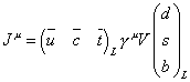
where V is the Kobayashi-Maskawa matrix. It’s also written KM-matrix, CKM-matrix, or U_KM

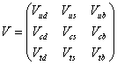
There is freedom in the matrix allowing permutation between various generations. You can fix this freedom by ordering the quarks by their masses. An n x n matrix has n² real parameters so there is further freedom in the phase structure in the KM-matrix. You can fix this by demanding that the matrix have the minimum number of phases. In the three generations case, the KM-matrix has a single phase which is the source of the weak CP-violation. The KM-matrix can be parametrizated in different ways, the following being the standard way.

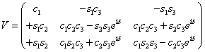
Here are the values derived from experiment.

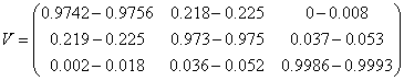
Here is an alternative parametrization proposed by Wolfenstein.

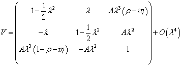
Since neutrinos have mass, there is a similar matrix relating their mass eigenstates to their flavour eigenstates, called the Maki-Nakagawa-Sakata matrix, which causes neutrino oscillation.

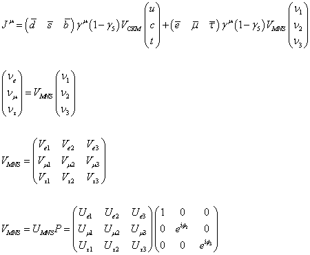
where P is the Majorana-phase matrix.

The term Yukawa coupling is a general term for an interaction term between fermions and scalars of the form

[psi bar][psi][phi]

At short distances, the gluon is the mediator of the strong force between quarks. This is the pure strong force. Gluons are confined to the same space to which quarks are confined. Thus, they never get out of the nucleon to create a force between one nucleon and another nucleon, such as in a nucleus, to bind the nucleus together. Therefore, gluons are useless for a long distance force, where long can be as short as 2 or 3 fermi. 1 fermi = 10^-15 meters.

However, mesons can exist outside nucleons and can, thus, be exchanged over larger distances as compared to gluons. Therefore, it is assumed that the strong interactions between nucleons in a nucleus is achieved by exchanging mesons, specifically the pion, as opposed to the strong interaction between quarks which is achieved by exchanging gluons. The creation of these pions goes back to processes between quarks and gluons that take place inside a nucleon. The meson-exchange force is not a fundamental force. It is a residual strong force, in contrast to the pure version of the strong force mentioned above. It is just a spin-off of complicated quark gluon processes. Therefore, meson-exchange forces are typically weaker than the pure gluon exchange between quarks. The idea of meson exchange goes back to the original belief that the pion was the mediator of the strong force. This later seemed ridiculous since π⁺ itself was supposed to be an up quark and down antiquark but we still use the idea today as a residual force that binds nucleons into a nucleus.

This is analogous to the fact that the pure electromagnetic force acts between protons and electrons inside the atom, confining them to an atom, while a weaker residual electromagnetic force acts between atoms, binding them together to form molecules.

Sometimes, in order to quantize the gauge theory you must add a gauge fixing term and the corresponding Faddeev-Popov term. The first term breaks the gauge symmetry and therefore removes the divergence of the functional integral. The second term improves the integration measure to provide correct predictions for gauge invariant observables. The Faddeev-Popov term includes auxiliary anti-commutative fields called the Faddeev-Popov ghosts. The general form of a gauge-fixing term is

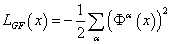
The corresponding Faddeev-Popov term is

where c^α and [c bar]_α are auxiliary anti-commutative fields called Faddeev-Popov ghosts. The most famous gauge-fixing term is the Feynman gauge.

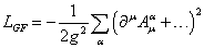
The corresponding Faddeev-Popov term is

After gauge fixing, you can bring the path integral to a form which contains unphysical ghost fields. The path integral may also be shown to be manifestly independent of gauge fixing. Then the action has a symmetry resulting of the original gauge invariance, which is lost when gauge fixing, called BRST symmetry, named after Becchi, Rouet, Stora, and Tyupin. Physical arguments lead to the conclusion that only states invariant under the BRST symmetry are physical.

The Standard Model can be used to calculate various quantities which can then be tested by experiment. So far, all experimental data is consistent with the Standard Model. A typical high energy physics experiment measures cross sections. Cross sections measure the effective area of interaction between beam and target particles. Cross sections are measured in barns, where 1 barn = 10^-24 cm². Cross sections can be interpreted as a measure of the relative probabilities of different kinds of events. A high cross section corresponds to a highly probable event. A low cross section corresponds to a rare one.

Let’s say you have initial particles which interact in a process called resonant scattering, and then decay into final particles.

A + B → R → C + D

For instance, A and B could be an e⁺e^– or quark pair. R could be a W⁺, W^–, or Z⁰.

For simplicity, assume spinless particles. The partial wave expansion of a scattering amplitude is

f([theta]) = (1/2ik)[summation over l](2l + 1)(e^2i[delta]_l -1)(P_l (cos [theta])

where k is the wavenumber which is the magnitude of the center of mass three momentum, and δ_l is the change in phase at the lth partial wave. “l” is lower case L. Again, I’m going to skip the algebra, but you eventually get the following relation for the cross section.

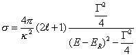
[sigma] = (4[pi]/k²) (2l + 1) (([gamma]²/4)/((E – E_R)² + ([gamma]²/4))

where σ is the cross section, E is the total energy of the scattering particles, E_R is the energy of the resonance, and Γ measures the rate of change of δ_l near the resonance. The above equation describes a curve called a Briet-Wigner resonance. Γ is the full width at half maximum.

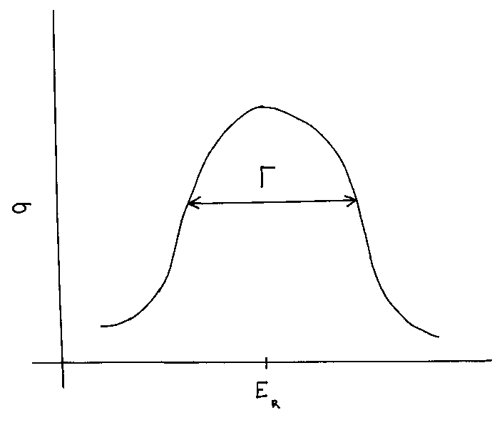
Let’s look at a more realistic case taking into account spin, color charge, and several final particles.

A + B → R → C + D + E…

The cross section is

[sigma] = (4[pi]s/k²)[(2S_R + 1)c_R)/((2s_A + 1)(2s_B)c_Ac_B)][([gamma]_AB^R[gamma]_f^R)/((s – m_R²)² + m_R²[gamma]_R²)]

where particles A and B scatter through resonance R, s is a Lorentz scalar variable, s_A is the spin of A, s_B is the spin of B, S_R is the spin of the resonance, c_A is the number of color charges of A, c_B is the number of color charges of B, c_R is the number of color charges of the resonance, m_R is the resonance mass, Γ_AB^R is the partial width for the reaction AB → R, and Γ_f^R is the partial width for R → final particles.

In electromagnetism, there exists a phenomenon called superconductivity. In the strong force, there exists an analogous phenomenon called color superconductivity. Superconductivity can only take place at low temperatures. Color superconductivity can only take place at very high pressures. The condensate is invariant only if you rotate color and flavor together which is called Color-Flavor Locking. Eight Goldstone bosons become the longitudinal components of the gluons which therefore become massive. At sufficiently high baryon densities, a nuclear matter will evolve to a quark matter. The attractive force mediated by one-gluon exchange or by instantons triggers the pairing instability and a color superconductor will be formed below a certain temperature. This phase of the nuclear matter may be found inside the core of a cold neutron star.

Here is a description of the Standard Model from the point of view of group theory.

Despite the enormous success of the Standard Model, it leaves many unanswered questions. There are many aspects of the Standard Model for which we would like a better explanation, and that point the way to possible extensions of the Standard Model.

The Standard Model has three different gauge groups and three coupling constants. It would be good if you could have a more unified gauge group, and understand the origin of the coupling constants. You should be able to predict sin² θ_w and the color gauge coupling α_s. These problems are addressed in grand unification. Why are left-handed fermions assigned to doublets, and right-handed fermions to singlets? Why are there three generations? Why do the masses exhibit a hierarchal pattern? The chirality of the fermions has to be put in by hand. The Higgs boson is the most obscure aspect of the Standard Model. You would hope that a more fundamental theory would explain the quantization of electric charge. Why is the electric charge of a down quark exactly 1/3 that of an electron? In grand unified theories, charge quantization follows automatically. Of course, ultimately we would like to include gravity in a fundamental theory of particle physics. Why is gravity so much weaker than the other forces?

Here is a list of some possible extensions of the Standard Model.

1. Axions, U(1) x SU(2) x SU(3) x U(1)_PQ Explains strong CP-violation. Predicts axion.

2. Majorons, familons, U(1) x SU(2) x SU(3) x U(1)_{B – L} This allows for small neutrino Majorana masses or possible quark mixing. Predicts majorons and familons.

3. Left-right symmetric models. Explains the origin of parity, CP-violation, quark mixing, possible small neutrino mass. Predicts new gauge bosons, heavy Majorana right-handed neutrino.

4. Supersymmetry, U(1) x SU(2) x SU(3) x SUSY Explains the hierarchy problem, Higgs mass, can possibly extend to gravity. Predicts supersymmetric partners.

5. Technicolor, U(1) x SU(2) x SU(3) x G_hypercolor Explains the hierarchy problem, Higgs mass. Predicts low mass neutral and charged Higgs bosons.

6. Grand Unified Theories, SU(5), SO(10), E₈, etc. Explains unification of gauge couplings. Predicts proton decay, neutron-antineutron oscillations.

7. Kaluza-Klein, Unifies gauge and equivalence principle. Attempts to unite gravity with other forces. Assumes existence of higher dimensions.

8. Superstrings, Unification of gravity with other forces in a locally supersymmetric higher dimensional theory. Explains fermion generations.

I’m going to briefly discuss the simplest grand unified theory, or GUT, which is SU(5). Howard Georgi and Sheldon Glashow invented the SU(5) model in 1974. It is possible to construct models which unify quarks and leptons, and which also unify the electroweak and strong force. Just as SU(2) is based on the doublet, SU(5) is based on the pentuplet, or 5-component object.

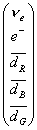
The top two are the SU(2)_Ldoublet. The bottom three are the color triplet [d_L bar]. Imagine the generators are matrices where the sum of the diagonal elements is zero. The particles from one family are contained in a mixture of these.

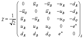
The Higgs sector, in which φ is a 5 x 5 matrix, acquires the following vacuum expectation value.

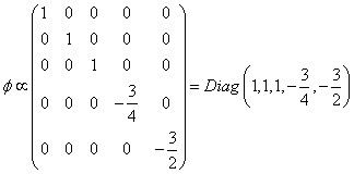
The charges of the particles in one SU(5) pentuplet add up to zero.

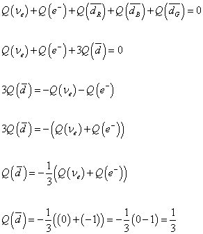
Q([nu]_e) + Q(e^–) + 3Q([d bar]) = 0

Q([d bar]) = -(1/3)(0 -1) = 1/3

The fractional charge of the quarks is related to the number of colors. Such an embedding of quarks and leptons into one simple group explains why the charge of the electron is of equal magnitude and opposite sign from that of the proton. It explains why charge is quantized, and why the hydrogen atom is electrically neutral.

The SU(5) model also explains the scaling of the coupling constants, and predicts they converge at some high energy scale. The SU(5) model also enables you to predict sin²θ_w.

An SU(n) theory has n² – 1 gauge bosons. Thus SU(5) has 5² – 1 = 24 gauge bosons. Twelve are the same as the Standard Model, which are the photon, three intermediate vector bosons, and the eight gluons. 1 + 3 + 8 = 12. There are also twelve new ones. They are an SU(2) doublet of color triplets and their antiparticles.

The X boson has an electric charge of -4/3, and the Y boson has a charge of -1/3. They each come in the three colors, red, blue, green, so that’s six particles. Then you have their antiparticles, which gives you a total of 12 new gauge bosons. The next simplest GUT is SO(10) which predicts a total of 45 gauge bosons which include the 24 in SU(5). The exchange of X and Y allows reactions that are not possible in the Standard Model.

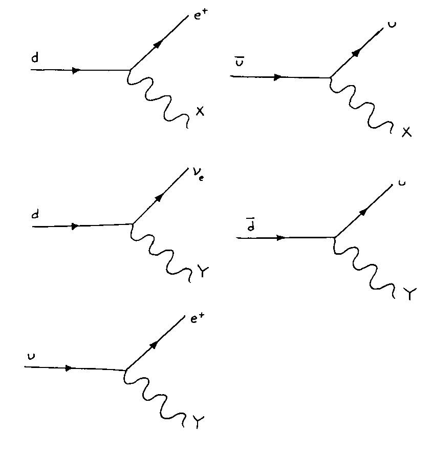
These reactions allow proton decay.

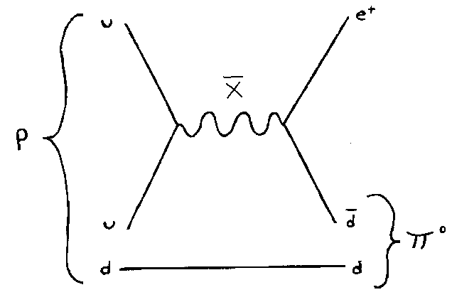
According to SU(5), the proton would have a lifetime of 10³⁰ years, which has already been ruled out by experiment. However, other grand unified theories, such as SO(10), predict longer proton lifetimes. Also, if you take SU(5) grand unified theory, and combine it with supersymmetry, it predicts a lifetime of 10³² – 10³³ years, which is not inconsistent with current experimental data.

Up until now, we have assumed that the symmetry of the S-matrix involved only commutators. If you allow both commutators and anticommutators, you have supersymmetry. It’s an extension of Poincare symmetry by anticommuting spinor generators. This is a weakening of the assumptions of the Coleman-Mandula theorem which says that the only allowed symmetries of the S-matrix are Poincare invariance, internal global symmetries related to conserved quantum numbers, and the C, P, and T symmetries. Supersymmetry was proposed independently by Gol’fand and Lichtman in 1971, Volkov and Akulov in 1972, and Wess and Zumino in 1974. The ultimate result is an operator that changes bosons to fermions, and the conjugate operator that changes fermions to bosons.

Q | b > = | f >

Obviously, supersymmetry is not an unbroken symmetry but it could be a broken symmetry. According to supersymmetry, every particle has a supersymmetric partner that has a spin that is ½ less. The partners of fermions begin with “s-“. The partners of bosons end with “-ino”. The supersymmetric partner of the electron is the selectron which has spin 0. The supersymmetric partner of the photon is the photino which has spin ½. The other quantum numbers are unchanged.

Just as with the fermions of the Standard Model, supersymmetry allows for the partners to have arbitrary masses, but does not predict the masses. To calculate in supersymmetry, you just take the Feynman rules from the Standard Model, and replace the particles with their supersymmetric partners, keeping the coupling constants the same. Supersymmetry allows the following vertices.

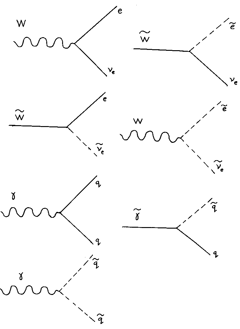
In supersymmetry, particles have a quantum number called R-parity. The particles we know about have even R-parity, and their superpartners have odd R-parity. Supersymmetric partners will be produced in pairs starting from normal particles. The decay of supersymmetric partners will contain at least one supersymmetric particle. The lightest supersymmetric particle will be stable. It’s often assumed to be the photino which is a candidate for dark matter.

The masses of the elementary particles are at an energy scale much lower than the GUT scale, 10¹⁴ GeV, or the Planck scale, 10¹⁹ GeV. You would expect that the self-energy due to virtual particles would drive up the masses. You can solve this by fine-tuning the parameters but in that case, they have to be fine-tuned to 26 decimal places which is unacceptable. This is called the hierarchy problem, and supersymmetry provides a solution. In supersymmetry, the contribution to the mass from every virtual particle would be exactly cancelled by an identical opposite contribution from its superpartner. The effects from the successive loop diagrams from bosons and fermions are exactly opposite and cancel out. This would keep the masses of the particles down to the experimentally measured values despite the large gap between the electroweak energy scale and the GUT scale. Also, it would keep the Higgs mass down to about 1 TeV. Much higher would violate unitarity. Therefore, the supersymmetry breaking scale is expected to be around 1 TeV. This predicts that the supersymmetric partners, as well as the Higgs, should be around that range, which will be accessible to the Large Hadron Collider at CERN. Also, if supersymmetry were an unbroken symmetry, which it obviously is not, these contributions to the vacuum energy from the equal number of bosons and fermions would exactly cancel out at all energy scales, and we would have no vacuum or zero point energy. However, supersymmetry is obviously not an unbroken symmetry.

In grand unified theories, the coupling constants get closer together and almost converge at higher and higher energies, which is the same thing as shorter and shorter distances, or farther back in time as you get closer and closer to the Big Bang. This is indirect evidence in favor of grand unified theories. Unfortunately, in grand unified theories, they get closer together but don’t actually converge. However, if you combine grand unified theories with supersymmetry, the coupling constants do exactly converge. This is another benefit of supersymmetry.

Throughout this paper, I have discussed three of the four forces, which are electromagnetism, the strong force, and the weak force. However, I have barely mentioned the fourth force, which is gravity. It is very difficult to come up with a gauge theory of gravity because in general, the infinities are non-renormalizable. However, we have finally achieved this with string theory. Up until this point, we have assumed that fundamental particles are zero-dimensional points. String theory is based on the premise that instead particles are one-dimensional line segments. At energies far below the Planck mass, 10¹⁹ GeV, you can’t resolve distances as short as the Planck length, 10^-35 m, which is the typical length of the strings, which is why for most purposes, you can approximate them as point particles. If the two endpoints of a string join to form a little loop, it’s called a closed string. If not, it’s called an open string. If the endpoint of an open string is fixed, it’s called a Dirichlet boundary condition. If it’s free to move, it’s called a Neumann boundary condition. They could be fixed in some dimensions but not others. In more recent theories, if the endpoint of an open string is fixed, the thing it’s fixed to is called a D-brane.

String theory was originally invented in the early 1960’s by Gabriele Veneziano, and was applied to hadrons as an attempt to explain the strong force. In 1974, John Schwarz and Joel Scherk realized that string theory included a massless spin-2 particle that could be identified with the graviton, thus raising the possibility of uniting gravity with the other forces.

The reason gravity is non-renormalizable is because of the sharp corners at the vertices of the Feynman diagrams. However, in string theory, the Feynman diagrams are three-dimensional diagrams of tubes instead of lines, and are smooth without corners. This allows gravity to be renormalizable. If you combine supersymmetry with string theory, you have superstring theory. In non-supersymmetric string theory, there are 26 dimensions. In superstring theory, there are 10 dimensions, one time dimension, and nine spatial dimensions. The ones we don’t see are compactified on a type of space called a Calabi-Yau manifold. There are five types of string theory, which are Type I, Type IIA, Type IIB, and two heterotic strings, which have SO(32), and E₈ x E₈ symmetry respectively. Type I is an open string theory, and the rest are closed string theories. Type I has SO(32) symmetry. Type IIA and IIB do not have gauge symmetry. Type IIA is parity conserving, in contradiction to reality, although it can be made parity violating through compactification. When a string vibrates or oscillates in different ways, it appears like different particles. On heterotic strings, the vibrations moving in one direction are non-supersymmetric, and those moving in the other direction are supersymmetric, instead of both being supersymmetric. For a while, the E₈ x E₈ heterotic string compactified on a Calabi-Yau manifold, appeared to be the best hope since it produced a low-energy effective theory that matched a supersymmetric extension of the Standard Model.

It now appears that all the different versions of string theory are actually just different manifestations of a more fundamental theory called M-theory. There is also another theory that has 11 dimensions that in addition to the five string theories, also reduces to the underlying M-theory. Unfortunately, this 11-dimensional supergravity theory is also often called M-theory. It should be emphasized that the 11-dimensional supergravity theory is not any more fundamental than the five string theories, but they are all different manifestations or solutions of a fundamental theory usually called M-theory.